Example to illustrate idea that likelihood ratio must be computed from same data
Matthew Stephens
2016-09-04
Last updated: 2019-03-31
Checks: 6 0
Knit directory: fiveMinuteStats/analysis/
This reproducible R Markdown analysis was created with workflowr (version 1.2.0). The Report tab describes the reproducibility checks that were applied when the results were created. The Past versions tab lists the development history.
Great! Since the R Markdown file has been committed to the Git repository, you know the exact version of the code that produced these results.
Great job! The global environment was empty. Objects defined in the global environment can affect the analysis in your R Markdown file in unknown ways. For reproduciblity it’s best to always run the code in an empty environment.
The command set.seed(12345) was run prior to running the code in the R Markdown file. Setting a seed ensures that any results that rely on randomness, e.g. subsampling or permutations, are reproducible.
Great job! Recording the operating system, R version, and package versions is critical for reproducibility.
Nice! There were no cached chunks for this analysis, so you can be confident that you successfully produced the results during this run.
Great! You are using Git for version control. Tracking code development and connecting the code version to the results is critical for reproducibility. The version displayed above was the version of the Git repository at the time these results were generated.
Note that you need to be careful to ensure that all relevant files for the analysis have been committed to Git prior to generating the results (you can use wflow_publish or wflow_git_commit). workflowr only checks the R Markdown file, but you know if there are other scripts or data files that it depends on. Below is the status of the Git repository when the results were generated:
Ignored files:
    Ignored:    .Rhistory
    Ignored:    .Rproj.user/
    Ignored:    analysis/.Rhistory
    Ignored:    analysis/bernoulli_poisson_process_cache/

Untracked files:
    Untracked:  _workflowr.yml
    Untracked:  analysis/CI.Rmd
    Untracked:  analysis/gibbs_structure.Rmd
    Untracked:  analysis/libs/
    Untracked:  analysis/results.Rmd
    Untracked:  analysis/shiny/tester/
    Untracked:  docs/MH_intro_files/
    Untracked:  docs/citations.bib
    Untracked:  docs/hmm_files/
    Untracked:  docs/libs/
    Untracked:  docs/shiny/tester/
Note that any generated files, e.g. HTML, png, CSS, etc., are not included in this status report because it is ok for generated content to have uncommitted changes.
These are the previous versions of the R Markdown and HTML files. If you’ve configured a remote Git repository (see ?wflow_git_remote), click on the hyperlinks in the table below to view them.
| File | Version | Author | Date | Message |
|---|---|---|---|---|
| html | 34bcc51 | John Blischak | 2017-03-06 | Build site. |
| Rmd | 5fbc8b5 | John Blischak | 2017-03-06 | Update workflowr project with wflow_update (version 0.4.0). |
| Rmd | 391ba3c | John Blischak | 2017-03-06 | Remove front and end matter of non-standard templates. |
| html | fb0f6e3 | stephens999 | 2017-03-03 | Merge pull request #33 from mdavy86/f/review |
| html | c3b365a | John Blischak | 2017-01-02 | Build site. |
| Rmd | 67a8575 | John Blischak | 2017-01-02 | Use external chunk to set knitr chunk options. |
| Rmd | 5ec12c7 | John Blischak | 2017-01-02 | Use session-info chunk. |
| Rmd | ae24830 | stephens999 | 2016-09-04 | add example of computing LR on different data |
Pre-requisites
- Likelihood Ratio.
Example
Suppose that we are considering whether to model some data \(X\) as normal or log-normal. In this case we’ll assume the truth is that the data are log normal, which we can simulate as follows:
X = exp(rnorm(1000,-5,2))We will use \(Z\) to denote \(\log(X)\):
Z = log(X)And let’s check by graphing which looks more normal:
par(mfcol=c(2,2))
hist(X)
hist(Z)
qqnorm(X)
qqnorm(Z)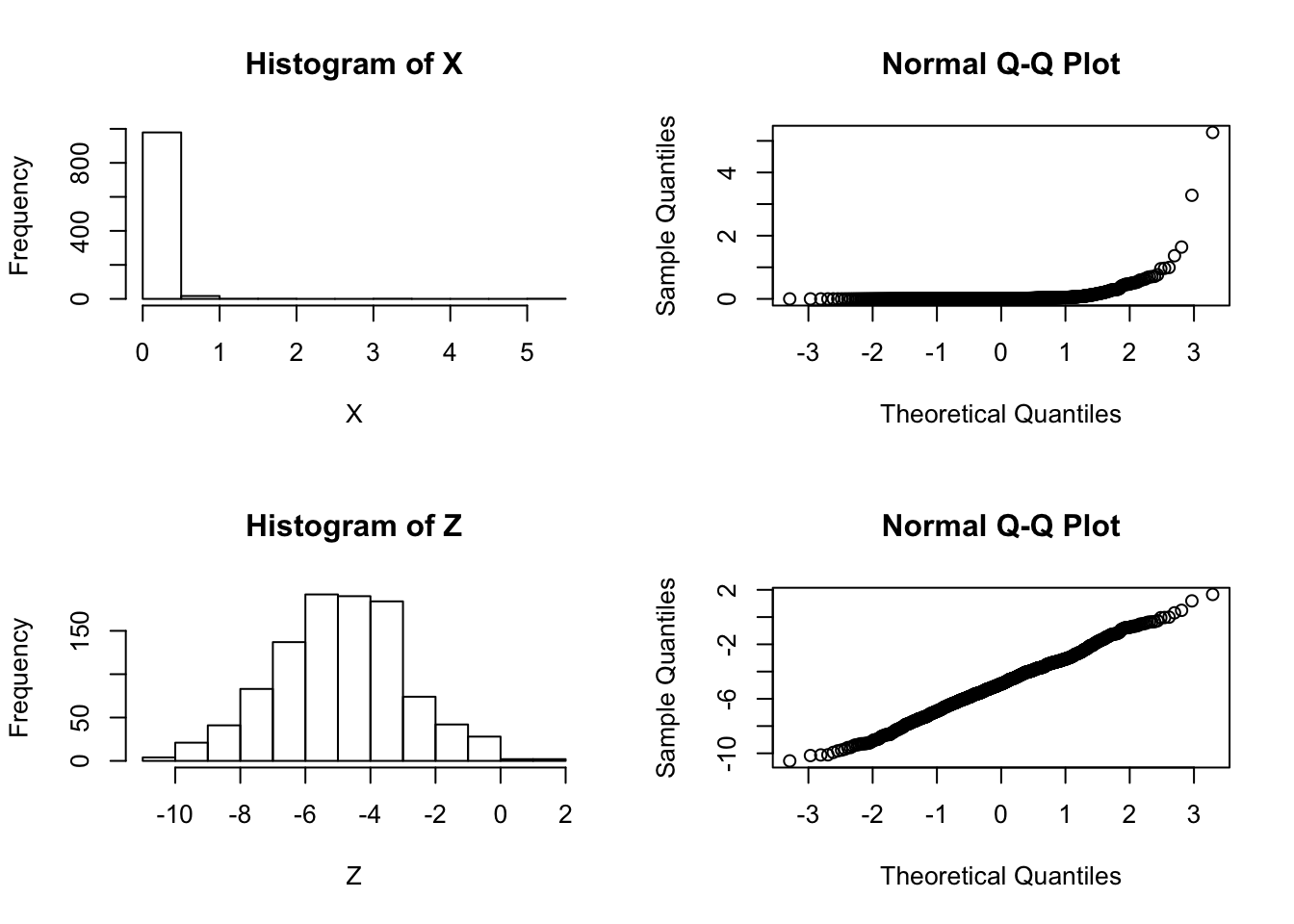
| Version | Author | Date |
|---|---|---|
| c3b365a | John Blischak | 2017-01-02 |
So it is pretty clear that the model ``\(M_2: \log(X)\) is normal" is better than the model “\(M_1: X\) is normal”.
Now consider computing a “log-likelihood” for each model.
To compute a log-likelihood under the model “X is normal” we need to also specify a mean and variance (or standard deviation). We use the sample mean and variance here:
sum(dnorm(X, mean=mean(X), sd=sd(X),log=TRUE))[1] 43.45732Doing the same for \(Z\) we obtain:
sum(dnorm(Z, mean=mean(Z), sd=sd(Z),log=TRUE))[1] -2110.333Done this way the log-likelihood for \(M_1\) appears much larger than the log-likelihood for \(M_2\), contradicting both the graphical evidence and the way the data were simulated.
The right way
The explanation here is that it does not make sense to compare a likelihood for \(Z\) with a likelihood for \(X\) because even though \(Z\) and \(X\) are 1-1 mappings of one another (\(Z\) is determined by \(X\), and vice versa), they are formally not the same data. That is, it does not make sense to compute \[\text{"LLR"} := \log(p(X|M_1)/p(Z|M_2))\].
However, we could compute a log-likelihood ratio for this problem as \[\text{LLR} := log(p(X|M_1)/p(X|M_2)).\] Here we are using the fact that the model \(M_2\) for \(Z\) actually implies a model for \(X\): \(Z\) is normal if and only if \(X\) is log-normal. So a sensible LLR would be given by:
sum(dnorm(X, mean=mean(X), sd=sd(X),log=TRUE)) - sum(dlnorm(X, meanlog=mean(Z), sdlog=sd(Z),log=TRUE))[1] -2753.814The fact that the LLR is very negative supports the graphical evidence that \(M_2\) is a much better fitting model (and indeed, as we know – since we simulated the data – \(M_2\) is the true model).
sessionInfo()R version 3.5.2 (2018-12-20)
Platform: x86_64-apple-darwin15.6.0 (64-bit)
Running under: macOS Mojave 10.14.1
Matrix products: default
BLAS: /Library/Frameworks/R.framework/Versions/3.5/Resources/lib/libRblas.0.dylib
LAPACK: /Library/Frameworks/R.framework/Versions/3.5/Resources/lib/libRlapack.dylib
locale:
[1] en_US.UTF-8/en_US.UTF-8/en_US.UTF-8/C/en_US.UTF-8/en_US.UTF-8
attached base packages:
[1] stats graphics grDevices utils datasets methods base
loaded via a namespace (and not attached):
[1] workflowr_1.2.0 Rcpp_1.0.0 digest_0.6.18 rprojroot_1.3-2
[5] backports_1.1.3 git2r_0.24.0 magrittr_1.5 evaluate_0.12
[9] stringi_1.2.4 fs_1.2.6 whisker_0.3-2 rmarkdown_1.11
[13] tools_3.5.2 stringr_1.3.1 glue_1.3.0 xfun_0.4
[17] yaml_2.2.0 compiler_3.5.2 htmltools_0.3.6 knitr_1.21 This site was created with R Markdown