The Metropolis Hastings Algorithm 2
Matthew Stephens
2022-04-26
Last updated: 2022-04-26
Checks: 7 0
Knit directory: fiveMinuteStats/analysis/
This reproducible R Markdown analysis was created with workflowr (version 1.7.0). The Checks tab describes the reproducibility checks that were applied when the results were created. The Past versions tab lists the development history.
Great! Since the R Markdown file has been committed to the Git repository, you know the exact version of the code that produced these results.
Great job! The global environment was empty. Objects defined in the global environment can affect the analysis in your R Markdown file in unknown ways. For reproduciblity it’s best to always run the code in an empty environment.
The command set.seed(12345) was run prior to running the code in the R Markdown file. Setting a seed ensures that any results that rely on randomness, e.g. subsampling or permutations, are reproducible.
Great job! Recording the operating system, R version, and package versions is critical for reproducibility.
Nice! There were no cached chunks for this analysis, so you can be confident that you successfully produced the results during this run.
Great job! Using relative paths to the files within your workflowr project makes it easier to run your code on other machines.
Great! You are using Git for version control. Tracking code development and connecting the code version to the results is critical for reproducibility.
The results in this page were generated with repository version cf196e8. See the Past versions tab to see a history of the changes made to the R Markdown and HTML files.
Note that you need to be careful to ensure that all relevant files for the analysis have been committed to Git prior to generating the results (you can use wflow_publish or wflow_git_commit). workflowr only checks the R Markdown file, but you know if there are other scripts or data files that it depends on. Below is the status of the Git repository when the results were generated:
Ignored files:
    Ignored:    .Rhistory
    Ignored:    .Rproj.user/
    Ignored:    analysis/.Rhistory
    Ignored:    analysis/bernoulli_poisson_process_cache/
    Ignored:    data/

Untracked files:
    Untracked:  _workflowr.yml
    Untracked:  analysis/CI.Rmd
    Untracked:  analysis/gibbs_structure.Rmd
    Untracked:  analysis/libs/
    Untracked:  analysis/results.Rmd
    Untracked:  analysis/shiny/tester/
    Untracked:  analysis/stan_8schools.Rmd

Unstaged changes:
    Modified:   analysis/LR_and_BF.Rmd
    Modified:   analysis/MH-examples1.Rmd
    Modified:   analysis/MH_intro.Rmd
    Deleted:    analysis/r_simplemix_extended.Rmd
Note that any generated files, e.g. HTML, png, CSS, etc., are not included in this status report because it is ok for generated content to have uncommitted changes.
These are the previous versions of the repository in which changes were made to the R Markdown (analysis/MH_intro_02.Rmd) and HTML (docs/MH_intro_02.html) files. If you’ve configured a remote Git repository (see ?wflow_git_remote), click on the hyperlinks in the table below to view the files as they were in that past version.
| File | Version | Author | Date | Message |
|---|---|---|---|---|
| Rmd | cf196e8 | Matthew Stephens | 2022-04-26 | workflowr::wflow_publish(“MH_intro_02.Rmd”) |
Prerequisites
You should be familiar with the Metropolis–Hastings algorithm.
Introduction
In this vignette we follow up on the original algorithm with a couple of points: numerical issues that were glossed over, and a useful plot.
Avoiding numerical issues in acceptance probability
The key to the MH algorithm is computing the acceptance probability, which recall is given by \[A= \min \left( 1, \frac{\pi(y)Q(x_t | y)}{\pi(x_t)Q(y | x_t)} \right).\]
In practice both terms in the fraction may be very close to 0, so on a computer you should do this computation on the logarithmic scale before exponentiating; something like this: \[\frac{\pi(y)Q(x_t | y)}{\pi(x_t)Q(y | x_t)} = \exp\left[ \log\pi(y) + \log Q(x_t | y) - \log \pi(x_t) - \log Q(y | x_t) \right]\]
Furthermore, the log values in this expression should be computed directly, and not by computing them and then taking the log. For example, in our previous example we sampled from a target distribution that was the exponential: \[\pi(x) = \exp(-x) \qquad (x>0)\] we we can directly compute \(\log \pi(x) = -x\). The code we had in that previous example can therefore be written as follows:
log_target = function(x){
  return(ifelse(x<0,-Inf,-x))
}

x = rep(0,10000)
x[1] = 100     #initialize; For purposes of illustration I set this to 100
for(i in 2:10000){
  current_x = x[i-1]
  proposed_x = current_x + rnorm(1,mean=0,sd=1)
  A = exp(log_target(proposed_x) - log_target(current_x) )
  if(runif(1)<A){
    x[i] = proposed_x       # accept move with probabily min(1,A)
  } else {
    x[i] = current_x        # otherwise "reject" move, and stay where we are
  }
}
An important and useful plot
In practice MCMC is usually performed in high dimensional space. It can therefore be really hard to visualize directly the values of the chain. A simple 1-d summary that is always available is the log-target density, \(\log \pi(x)\). So you should usually plot a trace of this whenever you run an MCMC scheme.
plot(log_target(x), main = "log-target value")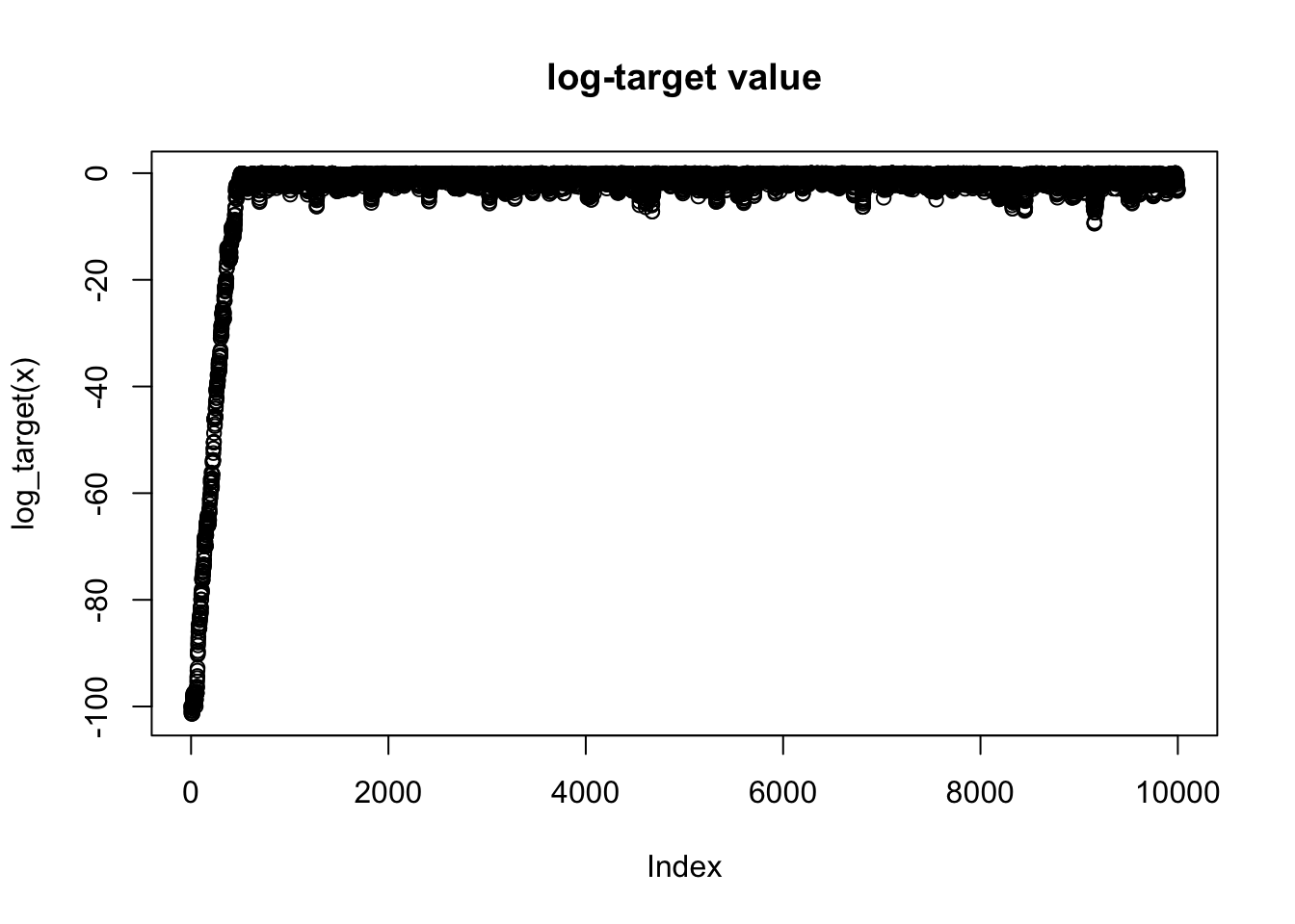
Here the plot shows “typical” behaviour of MCMC scheme: because the starting point is chosen not to be close to the optimal of \(\pi\), the chain initially takes some iterations to find a part of the space where \(\pi(x)\) is ``large". Once it finds that part of the space it starts to explore around the region where \(\pi(x)\) is large.
Burn-in
The plot in the previous section immediately shows that there is an initial period of time where the Markov Chain is unduly influenced by its starting position. In other words, during those iterations the Markov Chain has not “converged” and those samples should not be considered to be samples from \(\pi\). To address this it is common to discard the first set of iterations of any chain; the iterations that are discarded are often called “burn-in”.
Here, based on the plot we might discard the first 1000 iterations or so as burn-in. Here are comparisons of the samples with and without burnin discarded:
hist(x, main="without burn-in discarded")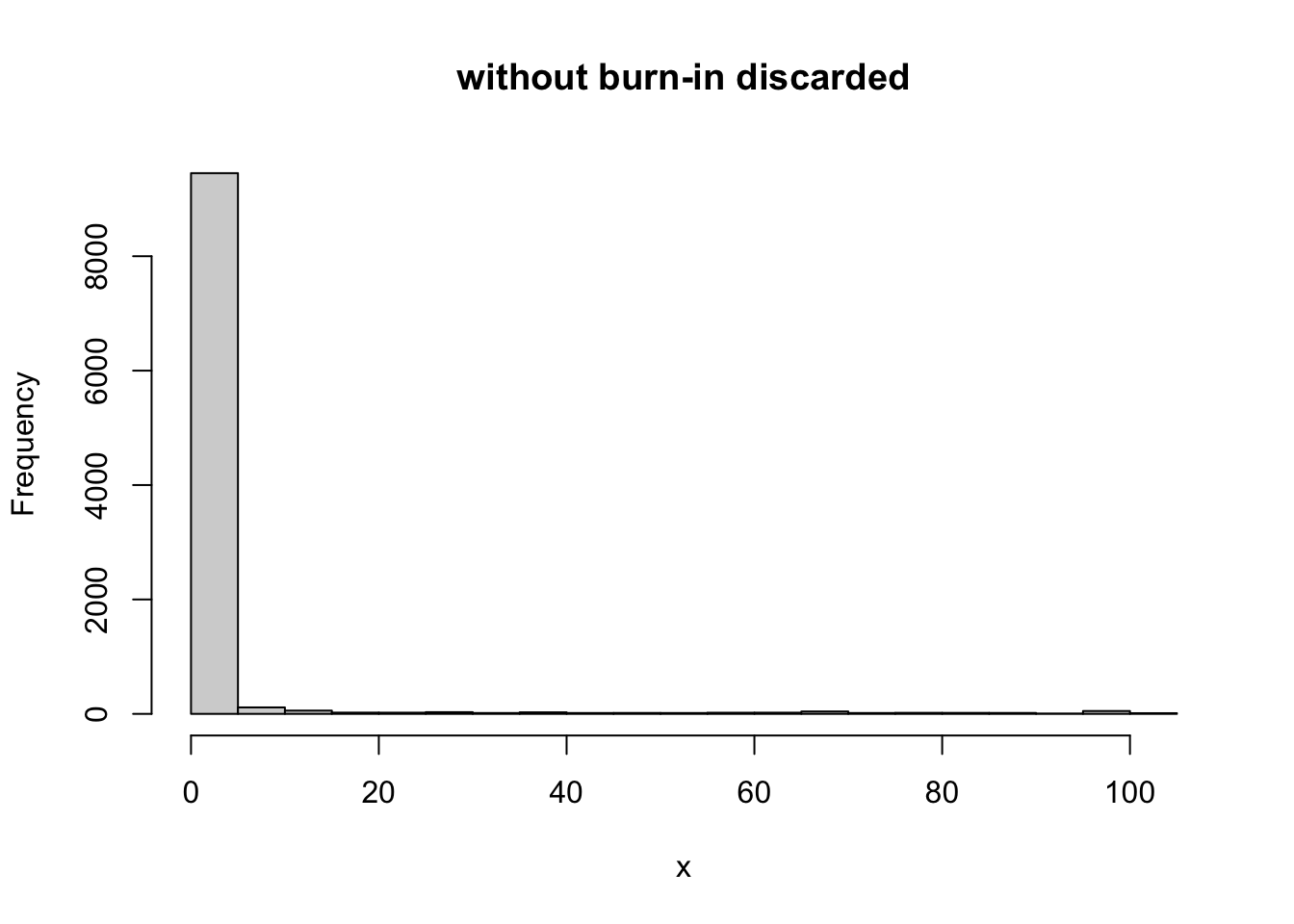
hist(x[-(1:1000)], main="with burn-in discarded")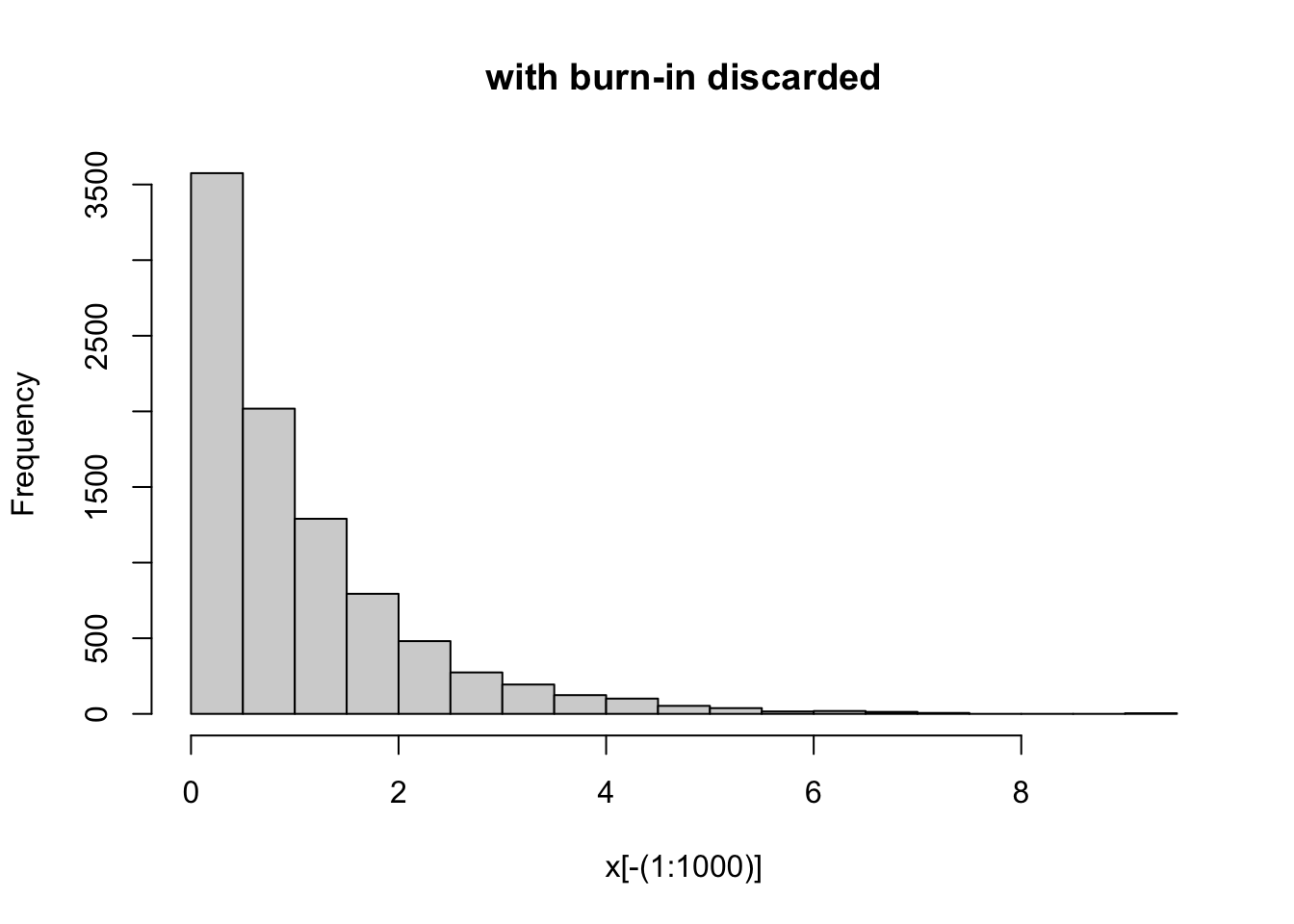
sessionInfo()R version 4.1.0 Patched (2021-07-20 r80657)
Platform: aarch64-apple-darwin20 (64-bit)
Running under: macOS Monterey 12.2
Matrix products: default
BLAS: /Library/Frameworks/R.framework/Versions/4.1-arm64/Resources/lib/libRblas.0.dylib
LAPACK: /Library/Frameworks/R.framework/Versions/4.1-arm64/Resources/lib/libRlapack.dylib
locale:
[1] en_US.UTF-8/en_US.UTF-8/en_US.UTF-8/C/en_US.UTF-8/en_US.UTF-8
attached base packages:
[1] stats graphics grDevices utils datasets methods base
loaded via a namespace (and not attached):
[1] Rcpp_1.0.7 whisker_0.4 knitr_1.36 magrittr_2.0.2
[5] workflowr_1.7.0 R6_2.5.1 rlang_0.4.12 fastmap_1.1.0
[9] fansi_0.5.0 highr_0.9 stringr_1.4.0 tools_4.1.0
[13] xfun_0.28 utf8_1.2.2 git2r_0.29.0 jquerylib_0.1.4
[17] htmltools_0.5.2 ellipsis_0.3.2 rprojroot_2.0.2 yaml_2.2.1
[21] digest_0.6.28 tibble_3.1.6 lifecycle_1.0.1 crayon_1.4.2
[25] later_1.3.0 sass_0.4.1 vctrs_0.3.8 fs_1.5.0
[29] promises_1.2.0.1 glue_1.5.0 evaluate_0.14 rmarkdown_2.11
[33] stringi_1.7.5 bslib_0.3.1 compiler_4.1.0 pillar_1.6.4
[37] jsonlite_1.7.2 httpuv_1.6.3 pkgconfig_2.0.3 This site was created with R Markdown