Asymptotic Normality of MLE
Matt Bonakdarpour [cre], Joshua Bon [ctb], Matthew Stephens [ctb]
2019-03-30
Last updated: 2020-01-11
Checks: 7 0
Knit directory: fiveMinuteStats/analysis/
This reproducible R Markdown analysis was created with workflowr (version 1.6.0). The Checks tab describes the reproducibility checks that were applied when the results were created. The Past versions tab lists the development history.
Great! Since the R Markdown file has been committed to the Git repository, you know the exact version of the code that produced these results.
Great job! The global environment was empty. Objects defined in the global environment can affect the analysis in your R Markdown file in unknown ways. For reproduciblity it’s best to always run the code in an empty environment.
The command set.seed(12345) was run prior to running the code in the R Markdown file. Setting a seed ensures that any results that rely on randomness, e.g. subsampling or permutations, are reproducible.
Great job! Recording the operating system, R version, and package versions is critical for reproducibility.
Nice! There were no cached chunks for this analysis, so you can be confident that you successfully produced the results during this run.
Great job! Using relative paths to the files within your workflowr project makes it easier to run your code on other machines.
Great! You are using Git for version control. Tracking code development and connecting the code version to the results is critical for reproducibility. The version displayed above was the version of the Git repository at the time these results were generated.
Note that you need to be careful to ensure that all relevant files for the analysis have been committed to Git prior to generating the results (you can use wflow_publish or wflow_git_commit). workflowr only checks the R Markdown file, but you know if there are other scripts or data files that it depends on. Below is the status of the Git repository when the results were generated:
Ignored files:
    Ignored:    .Rhistory
    Ignored:    .Rproj.user/
    Ignored:    analysis/.Rhistory
    Ignored:    analysis/bernoulli_poisson_process_cache/

Untracked files:
    Untracked:  _workflowr.yml
    Untracked:  analysis/CI.Rmd
    Untracked:  analysis/gibbs_structure.Rmd
    Untracked:  analysis/libs/
    Untracked:  analysis/results.Rmd
    Untracked:  analysis/shiny/tester/
Note that any generated files, e.g. HTML, png, CSS, etc., are not included in this status report because it is ok for generated content to have uncommitted changes.
These are the previous versions of the R Markdown and HTML files. If you’ve configured a remote Git repository (see ?wflow_git_remote), click on the hyperlinks in the table below to view them.
| File | Version | Author | Date | Message |
|---|---|---|---|---|
| html | 2022f7f | Matthew Stephens | 2020-01-11 | Build site. |
| Rmd | 47f2119 | GitHub | 2019-12-13 | “Asymptotic normality” correct formal limit result |
| html | 4ba6ab1 | Matthew Stephens | 2019-03-31 | Build site. |
| Rmd | ad69a82 | Matthew Stephens | 2019-03-31 | workflowr::wflow_publish(“analysis/asymptotic_normality_mle.Rmd”) |
| html | 93f7225 | Matthew Stephens | 2019-03-31 | Build site. |
| Rmd | f6fd600 | Matthew Stephens | 2019-03-31 | workflowr::wflow_publish(“analysis/asymptotic_normality_mle.Rmd”) |
| html | 5f62ee6 | Matthew Stephens | 2019-03-31 | Build site. |
| Rmd | 0cd28bd | Matthew Stephens | 2019-03-31 | workflowr::wflow_publish(all = TRUE) |
| html | 0cd28bd | Matthew Stephens | 2019-03-31 | workflowr::wflow_publish(all = TRUE) |
| Rmd | 692af91 | Matthew Stephens | 2019-03-31 | some improvements to presentation of these results |
| Rmd | 4ed2708 | Joshua Bon | 2019-03-30 | Updates to Fisher information matrix, to distinguish between one-observation and all-sample versions. |
| html | 34bcc51 | John Blischak | 2017-03-06 | Build site. |
| Rmd | 5fbc8b5 | John Blischak | 2017-03-06 | Update workflowr project with wflow_update (version 0.4.0). |
| Rmd | 391ba3c | John Blischak | 2017-03-06 | Remove front and end matter of non-standard templates. |
| html | 8e61683 | Marcus Davy | 2017-03-03 | rendered html using wflow_build(all=TRUE) |
| Rmd | d674141 | Marcus Davy | 2017-02-26 | typos, refs |
| html | c3b365a | John Blischak | 2017-01-02 | Build site. |
| Rmd | 67a8575 | John Blischak | 2017-01-02 | Use external chunk to set knitr chunk options. |
| Rmd | 5ec12c7 | John Blischak | 2017-01-02 | Use session-info chunk. |
| Rmd | e33f3a5 | mbonakda | 2016-01-15 | remove keep_md. figures are saved without it enabled. |
| Rmd | b20215f | mbonakda | 2016-01-15 | remove keep_md |
| Rmd | 3bcbe0d | mbonakda | 2016-01-14 | Merge branch ‘master’ into gh-pages |
| Rmd | 360c471 | mbonakda | 2016-01-14 | conform to template + ignore md files |
| Rmd | c922b38 | mbonakda | 2016-01-14 | keep md files for figures |
| Rmd | 56a4848 | mbonakda | 2016-01-14 | fix plots |
| Rmd | 8673a57 | mbonakda | 2016-01-14 | fix mathjax |
| Rmd | 3e7ba92 | mbonakda | 2016-01-14 | fix mathjax problem |
| Rmd | ff6b857 | mbonakda | 2016-01-12 | add asymptotic normality of MLE and wilks |
Prerequisites
You should be familiar with the concept of Likelihood function.
Overview
Maximum likelihood estimation is a popular method for estimating parameters in a statistical model. As its name suggests, maximum likelihood estimation involves finding the value of the parameter that maximizes the likelihood function (or, equivalently, maximizes the log-likelihood function). This value is called the maximum likelihood estimate, or MLE.
It seems natural to ask about the accuracy of an MLE: how far from the “true” value of the parameter can we expect the MLE to be? This vignette answers this question in a simple but important case: maximum likelihood estimation based on independent and identically distributed (i.i.d.) data from a model.
Asymptotic distribution of MLE for i.i.d. data
Set-up
Suppose we observe independent and identically distributed (i.i.d.) samples \(X_1,\ldots,X_n\) from a probability distribution \(p(\cdot; \theta)\) governed by a parameter \(\theta\) that is to be estimated. Then the likelihood for \(\theta\) is: \[L(\theta; X_1,\dots,X_n) := p(X_1,\ldots,X_n;\theta) = \prod_{i=1}^n p(X_i ; \theta).\] And the log-likelihood is: \[\ell(\theta; X_1,\dots,X_n):= \log L(\theta;X_1,\dots,X_n) = \sum_{i=1}^n \log p(X_i; \theta).\] Let \(\theta_0\) denote the true value of \(\theta\), and \(\hat{\theta}\) denote the maximum likelihood estimate (MLE). Because \(\ell\) is a monotonic function of \(L\) the MLE \(\hat{\theta}\) maximizes both \(L\) and \(\ell\). (In simple cases we typically find \(\hat{\theta}\) by differentiating the log-likelihood and solving \(\ell'(\theta;X_1,\dots,X_n)=0\).)
Result
Under some technical conditions that often hold in practice (often referred to as “regularity conditions”), and for \(n\) sufficiently large, we have the following approximate result: \[{\hat{\theta}} {\dot\sim} N(\theta_0,I_{n}(\theta_0)^{-1})\] where the precision (inverse variance), \(I_n(\theta_0)\), is a quantity known as the Fisher information, which is defined as \[I_{n}(\theta) := E_{\theta}\left[-\frac{d^2}{d\theta^2}\ell(\theta; X_1,\dots,X_n)\right].\] Notes:
- the notation \(\dot\sim\) means “approximately distributed as”.
- the expectation in the definition of \(I_n\) is with respect to the distribution of \(X_1,\dots,X_n\), \(p(X_1,\dots,X_n | \theta)\).
- The (negative) second derivative measures the curvature of a function, and so one can think of \(I_{n}(\theta)\) as measuring, on average, how curved the log-likelihood function is – or, in other words, how peaked the likelihood function is. The more peaked the likelihood function, the more information it contains, and the more precise the MLE will be.
With i.i.d. data the Fisher information can be easily shown to have the form \[I_n(\theta) = n I(\theta)\] where \(I(\theta)\) is the Fisher information for a single observation - that is, \(I(\theta) = I_1(\theta)\). [This follows from the fact that \(\ell\) is the sum of \(n\) terms, and from linearity of expectation: Exercise!]
A slightly more precise statement
For those that dislike the vagueness of the statement “for \(n\) sufficiently large”, the result can be written more formally as a limiting result as \(n \rightarrow \infty\):
\[I_n(\theta_0)^{0.5} (\hat{\theta} - \theta_0) \rightarrow N(0,1) \text{ as } n \rightarrow \infty\]
This kind of result, where sample size tends to infinity, is often referred to as an “asymptotic” result in statistics. So the result gives the “asymptotic sampling distribution of the MLE”.
While mathematically more precise, this way of writing the result is perhaps less intutive than the approximate statement above.
Interpretation
Sampling distribution
The interpretation of this result needs a little care. In particular, it is important to understand what it means to say that the MLE has a “distribution”, since for any given dataset \(X_1,\dots,X_n\) the MLE \(\hat{\theta}\) is just a number.
One way to think of this is to imagine sampling several data sets \(X_1,\dots,X_n\), rather than just one data set. Each data set would give us an MLE. Supppose we collect \(J\) datasets, and the \(j\)th dataset gives an MLE \(\hat{\theta}_j\). The distribution of the MLE means the distribution of these \(\hat{\theta}_j\) values. Essentially it tells us what a histogram of the \(\hat{\theta}_j\) values would look like. This distribution is often called the “sampling distribution” of the MLE to emphasise that it is the distribution one would get when sampling many different data sets. The concrete examples given below help illustrate this key idea.
Implication for estimation error
Notice that, because the mean of the sampling distribution of the MLE is the true value (\(\theta_0\)), the variance of the sampling distribution tells us how far we might expect the MLE to lie from the true value. Specifically the variance is, by definition, the expected squared distance of the MLE from the true value \(\theta_0\). Thus the standard deviation (square root of variance) gives the root mean squared error (RMSE) of the MLE.
For i.i.d. data the Fisher information \(I_n(\theta)=nI(\theta)\) and so increases linearly with \(n\) (see notes above). Consequently the variance decreases linearly with \(n\) and the RMSE decreases with \(n^0.5\). Thus, for example, to halve the RMSE we need to multiply sample size by 4.
This is a fundamental idea in statistics: for i.i.d. data (and under regularity conditions) estimation error in the MLE decreases as the square root of the sample size.
Example 1: Bernoulli Proportion
Assume we observe i.i.d. samples \(X_1,\ldots,X_n\) drawn from a Bernoulli\((p)\) distribution with true parameter \(p=p_0\). The log-likelihood is: \[\ell(p; X_1,\dots,X_n) = \sum_{i=1}^n [X_i\log{p} + (1-X_i)\log(1-p)]\] Setting the derivative equal to zero, we obtain:
\[\frac{d}{dp}\ell(p;X_1,\dots,X_n) = \sum_{i=1}^n
\left[ \frac{X_i}{p} - \frac{(1-X_i)}{1-p}\right].\]
Setting this derivative to 0 and solving for \(p\), gives that the MLE is the sample mean: \(\hat{p} = (1/n)\sum_{i=1}^n X_i\).
The second derivative with respect to \(p\) is:
\[\frac{d^2}{dp^2} \ell(p; X_1,\dots,X_n) = \sum_{i=1}^n
\left[ -\frac{X_i}{p^2} - \frac{(1-X_i)}{(1-p)^2} \right]\]
The Fisher information (for all observations) is therefore: \[I_{n}(p) = E\left[-\frac{d^2}{dp^2}\ell(p)\right] = \sum_{i=1}^n \left[ -\frac{E[X_i]}{p^2} - \frac{(1-E[X_i])}{(1-p)^2} \right] = \frac{n}{p(1-p)}.\] Notice that, as expected from the general result \(I_n(p)=nI_1(p)\), \(I_n(p)\) increases linearly with \(n\).
From the main result, we have that (for large \(n\)), \(\hat{p}\) is approximately \(N\left(p,\frac{p(1-p)}{n}\right)\). We illustrate this approximation in the simulation below.
The simulation samples \(J=7000\) sets of data \(X_1,\dots,X_n\). In each sample, we have \(n=100\) draws from a Bernoulli distribution with true parameter \(p_0=0.4\). We compute the MLE separately for each sample and plot a histogram of these 7000 MLEs. On top of this histogram, we plot the density of the theoretical asymptotic sampling distribution as a solid line.
num.iterations         <- 7000
p.truth                <- 0.4
num.samples.per.iter   <- 100
samples                <- numeric(num.iterations)
for(iter in seq_len(num.iterations)) {
  samples[iter] <- mean(rbinom(num.samples.per.iter, 1, p.truth))
}
hist(samples, freq=F)
curve(dnorm(x, mean=p.truth,sd=sqrt((p.truth*(1-p.truth)/num.samples.per.iter) )), .25, .55, lwd=2, xlab = "", ylab = "", add = T)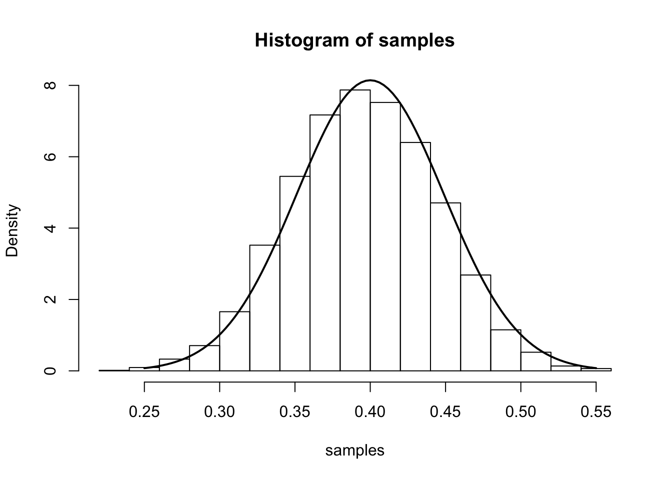
Example 2: Poisson Mean
Assume we observe i.i.d. samples \(X_1,\ldots,X_n\) drawn from a Poisson\((\lambda)\) distribution with true parameter \(\lambda=\lambda_0\). The log-likelihood is:
\[ \ell(\lambda; X_1,\ldots,X_n) = \sum_{i=1}^n -\lambda + X_i\log(\lambda) + \log(X_i!).\]
Taking the derivative with respect to \(\lambda\), setting it equal to zero, and solving for \(\lambda\) gives the mle as the sample mean, \(\hat{\lambda} = \frac{1}{n}\sum_{i=1}^{n}X_i\). The Fisher information is:
\[ I_{n}(\lambda) = E_{\lambda}\left[-\frac{d^2}{d\lambda^2}\ell(\lambda)\right] = \sum_{i=1}^n E[X_{i}/\lambda^2] = \frac{n}{\lambda}\]
The main result says that (for large \(n\)), \(\hat{\lambda}\) is approximately \(N\left(\lambda,\frac{1}{n\lambda}\right)\). We illustrate this by simulation again:
num.iterations         <- 7000
lambda.truth           <- 0.8
num.samples.per.iter   <- 100
samples                <- numeric(num.iterations)
for(iter in seq_len(num.iterations)) {
  samples[iter] <- mean(rpois(num.samples.per.iter, lambda.truth))
}
hist(samples, freq=F)
curve(dnorm(x, mean=lambda.truth,sd=sqrt(lambda.truth/num.samples.per.iter) ), 0.4, 1.2, lwd=2, xlab = "", ylab = "", add = T)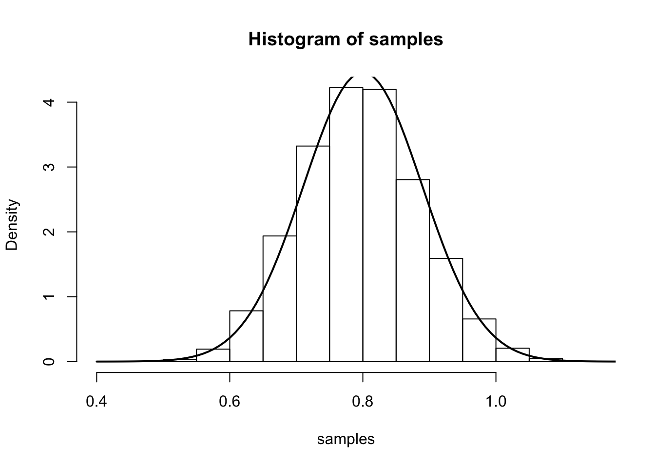
sessionInfo()R version 3.6.0 (2019-04-26)
Platform: x86_64-apple-darwin15.6.0 (64-bit)
Running under: macOS Mojave 10.14.6
Matrix products: default
BLAS: /Library/Frameworks/R.framework/Versions/3.6/Resources/lib/libRblas.0.dylib
LAPACK: /Library/Frameworks/R.framework/Versions/3.6/Resources/lib/libRlapack.dylib
locale:
[1] en_US.UTF-8/en_US.UTF-8/en_US.UTF-8/C/en_US.UTF-8/en_US.UTF-8
attached base packages:
[1] stats graphics grDevices utils datasets methods base
loaded via a namespace (and not attached):
[1] workflowr_1.6.0 Rcpp_1.0.3 rprojroot_1.3-2 digest_0.6.23
[5] later_1.0.0 R6_2.4.1 backports_1.1.5 git2r_0.26.1
[9] magrittr_1.5 evaluate_0.14 stringi_1.4.3 rlang_0.4.2
[13] fs_1.3.1 promises_1.1.0 whisker_0.4 rmarkdown_1.18
[17] tools_3.6.0 stringr_1.4.0 glue_1.3.1 httpuv_1.5.2
[21] xfun_0.11 yaml_2.2.0 compiler_3.6.0 htmltools_0.4.0
[25] knitr_1.26 This site was created with R Markdown