Linear combinations of independent normals are normal
Matthew Stephens
2022-03-01
Last updated: 2022-03-01
Checks: 7 0
Knit directory: fiveMinuteStats/analysis/
This reproducible R Markdown analysis was created with workflowr (version 1.7.0). The Checks tab describes the reproducibility checks that were applied when the results were created. The Past versions tab lists the development history.
Great! Since the R Markdown file has been committed to the Git repository, you know the exact version of the code that produced these results.
Great job! The global environment was empty. Objects defined in the global environment can affect the analysis in your R Markdown file in unknown ways. For reproduciblity it’s best to always run the code in an empty environment.
The command set.seed(12345) was run prior to running the code in the R Markdown file. Setting a seed ensures that any results that rely on randomness, e.g. subsampling or permutations, are reproducible.
Great job! Recording the operating system, R version, and package versions is critical for reproducibility.
Nice! There were no cached chunks for this analysis, so you can be confident that you successfully produced the results during this run.
Great job! Using relative paths to the files within your workflowr project makes it easier to run your code on other machines.
Great! You are using Git for version control. Tracking code development and connecting the code version to the results is critical for reproducibility.
The results in this page were generated with repository version 8ae5f5e. See the Past versions tab to see a history of the changes made to the R Markdown and HTML files.
Note that you need to be careful to ensure that all relevant files for the analysis have been committed to Git prior to generating the results (you can use wflow_publish or wflow_git_commit). workflowr only checks the R Markdown file, but you know if there are other scripts or data files that it depends on. Below is the status of the Git repository when the results were generated:
Ignored files:
    Ignored:    .Rhistory
    Ignored:    .Rproj.user/
    Ignored:    analysis/.Rhistory
    Ignored:    analysis/bernoulli_poisson_process_cache/

Untracked files:
    Untracked:  _workflowr.yml
    Untracked:  analysis/CI.Rmd
    Untracked:  analysis/gibbs_structure.Rmd
    Untracked:  analysis/libs/
    Untracked:  analysis/results.Rmd
    Untracked:  analysis/shiny/tester/

Unstaged changes:
    Modified:   analysis/LR_and_BF.Rmd
    Modified:   analysis/MH-examples1.Rmd
    Modified:   analysis/MH_intro.Rmd
    Deleted:    analysis/r_simplemix_extended.Rmd
Note that any generated files, e.g. HTML, png, CSS, etc., are not included in this status report because it is ok for generated content to have uncommitted changes.
These are the previous versions of the repository in which changes were made to the R Markdown (analysis/norm_linear_comb.Rmd) and HTML (docs/norm_linear_comb.html) files. If you’ve configured a remote Git repository (see ?wflow_git_remote), click on the hyperlinks in the table below to view the files as they were in that past version.
| File | Version | Author | Date | Message |
|---|---|---|---|---|
| Rmd | 8ae5f5e | Matthew Stephens | 2022-03-01 | workflowr::wflow_publish(“norm_linear_comb.Rmd”) |
Pre-requisites
Basic familiarity with the univariate normal distribution
A statement of the basic property
The simple goal of this vignette is to introduce a basic property of the (univariate) normal distribution: that linear combinations of independent normal variables are also normal.
Formally, suppose \(Z_1\) and \(Z_2\) represent independent, normally distributed random variables. Then for any scalars \(a\) and \(b\), the linear combination \[X:=aZ_1+bZ_2\] is also (univariate) normal.
Also, by basic properties of expectation and variance, \(E(X) = aE(Z_1)+bE(Z_2)\) and \(var(X)= a^2 var(Z_1) + b^2 var(Z_2)\).
Example
The following code provides a visual illustration of this idea with \(a=2\) and \(b=3\), but it holds for any \(a\) and \(b\).
First we sample some values of \(X\) by randomly generating \(Z_1\) and \(Z_2\), and computing \(X=aZ_1+bZ_2\):
Z1 = rnorm(1000)
Z2 = rnorm(1000)
a = 2
b = 3

X = a*Z1 + b*Z2
The property says that the samples of \(X\) look normal. A quick histogram and qqplot suggest it does…. (of course this is not a proof that the property holds; it is just an illustration of the idea).
hist(X)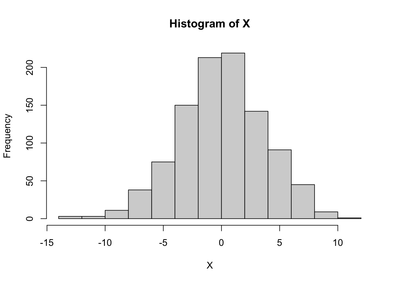
qqnorm(X)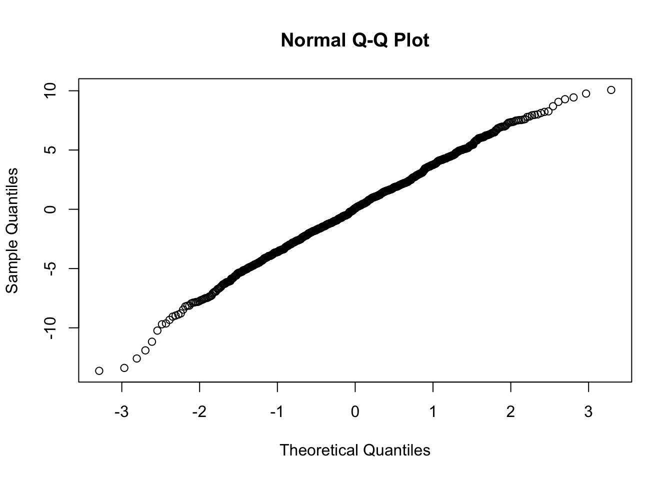
Addendum: Stable distributions
If you are curious by nature, you might now ask: is the normal distribution the only distribution that satisfies this property?
The answer is “no”. For example, \(t\) distributions also satisfy this property. Distributions that satisfy this property are called ``stable" distributions. You can read more at [https://en.wikipedia.org/wiki/Stable_distribution]
sessionInfo()R version 4.1.0 Patched (2021-07-20 r80657)
Platform: aarch64-apple-darwin20 (64-bit)
Running under: macOS Monterey 12.2
Matrix products: default
BLAS: /Library/Frameworks/R.framework/Versions/4.1-arm64/Resources/lib/libRblas.0.dylib
LAPACK: /Library/Frameworks/R.framework/Versions/4.1-arm64/Resources/lib/libRlapack.dylib
locale:
[1] en_US.UTF-8/en_US.UTF-8/en_US.UTF-8/C/en_US.UTF-8/en_US.UTF-8
attached base packages:
[1] stats graphics grDevices utils datasets methods base
loaded via a namespace (and not attached):
[1] Rcpp_1.0.7 whisker_0.4 knitr_1.36 magrittr_2.0.2
[5] workflowr_1.7.0 R6_2.5.1 rlang_0.4.12 fastmap_1.1.0
[9] fansi_0.5.0 highr_0.9 stringr_1.4.0 tools_4.1.0
[13] xfun_0.28 utf8_1.2.2 git2r_0.29.0 jquerylib_0.1.4
[17] htmltools_0.5.2 ellipsis_0.3.2 rprojroot_2.0.2 yaml_2.2.1
[21] digest_0.6.28 tibble_3.1.6 lifecycle_1.0.1 crayon_1.4.2
[25] later_1.3.0 vctrs_0.3.8 fs_1.5.0 promises_1.2.0.1
[29] glue_1.5.0 evaluate_0.14 rmarkdown_2.11 stringi_1.7.5
[33] compiler_4.1.0 pillar_1.6.4 httpuv_1.6.3 pkgconfig_2.0.3 This site was created with R Markdown