A quick look at the CCR5 data
Matthew Stephens and Peter Carbonetto
This is for Problem Set 7, Part B. See also Novembre et al 2005.
Load some packages used in the analysis below:
library(geosphere)
library(ggplot2)
library(cowplot)
library(maps)
library(mvtnorm)
Load the CCR5 data:
ccr5 <- read.table("../data/CCR5/CCR5.freq.txt",header = TRUE)Plot the distribution of allele frequencies:
hist(ccr5$Freq,breaks = 16)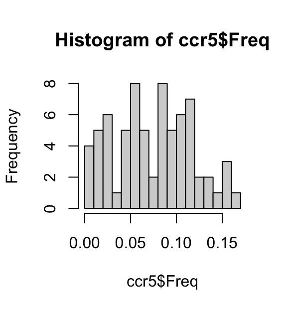
Change longitudes greater than 180 to negative numbers:
ccr5$Long <- ifelse(ccr5$Long > 180,ccr5$Long - 360,ccr5$Long)We will use this function below to plot the allele frequencies on a map of Europe (and parts of Asia):
draw_map <- function (dat)
  ggplot(dat,aes(x = Long,y = Lat)) +
    geom_path(data = map_data("world"),
              aes(x = long,y = lat,group = group),
              color = "gray",linewidth = 0.35) +
    xlim(c(-20,80)) +
    ylim(c(30,70)) +
    theme_cowplot(font_size = 12)
This plot shows the allele frequency data and the geographical locations where these data were obtained. Note that a few data points are not shown in this map.
draw_map(ccr5) +
  geom_point(shape = 21,color = "black",size = 2.5,
             mapping = aes(fill = Freq)) +
  scale_fill_gradient2(low = "deepskyblue",mid = "gold",high = "red",
                       midpoint = 0.1) +
  ggtitle("data")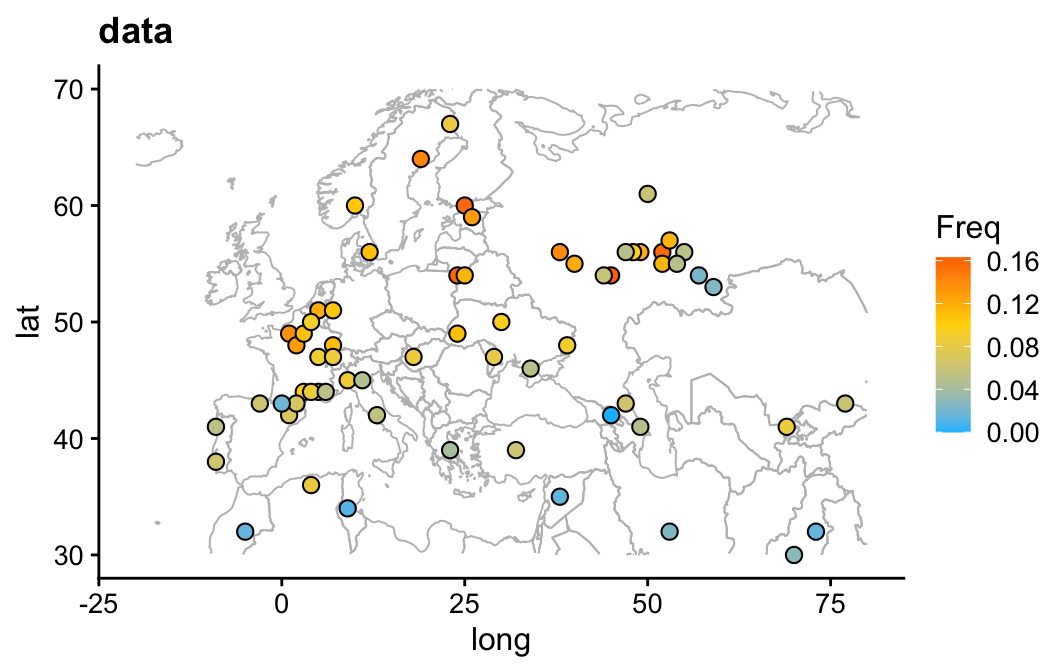
Compute pairwise distances
Compute distances (in km) between the points. Dividing by 1,000 gives distance in km.
D <- distm(ccr5[1:2])/1000
hist(D,breaks = 16,xlab = "distance (km)")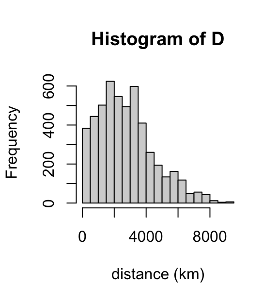
These distances seem to broadly make sense. For example, the driving distance from Paris to Moscow is about 3,000 km.
Deal with zero counts
Some of the frequency estimates are zero. I deal with this by first working out the original counts (2 * frequency * samplesize), and then adding a pseudocount to each allele before recomputing frequencies. The resulting column “fhat” can be transformed by log(fhat/(1-fhat)) to be something that is not entirely non-normal.
logit <- function (x) log(x/(1-x))
ccr5 <- transform(ccr5,count = round(2*Freq*SampleSize))
ccr5 <- transform(ccr5,fhat = (count + 1)/(2*SampleSize + 2))
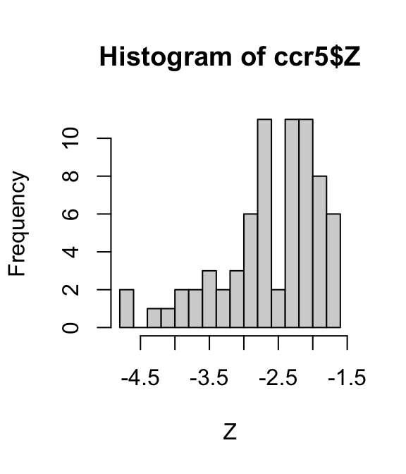
ccr5 <- transform(ccr5,Z = logit(fhat))
hist(ccr5$Z,breaks = 16,xlab = "Z")