A look at voom on simulated data, 2
M Stephens, modifying code from voom1.rmd by Mengyin Lu
2016-02-03
Last updated: 2016-02-04
Code version: cc743de0ed77120abe5ff470019987f7f7ba20fe
This does the same as voom1.html but with a different way of simulating the alternative genes. This is to test my hypothesis that the results in voom1.html are due to induced effects due to differences in library size. The crucial change is use of countmat3 instead of countmat2 below.
Define functions to generate an RNA-seq count matrix (with 2 conditions) and compute betahat (estimated effect size) & sebetahat (standard error):
library(limma)
library(edgeR)
library(qvalue)
Warning: replacing previous import by 'grid::arrow' when loading 'qvalue'Warning: replacing previous import by 'grid::unit' when loading 'qvalue'library(ashr)
# Generate count matrix
# counts 1 is G by N1
# counts 2 is G by N2
# note that unlike countmat2 it doesn't filter out low expressed genes - assumes this already done
countmat3 = function(counts1, counts2, Nnull, Nalt, Nsamp){
if(nrow(counts1)!=nrow(counts2)){stop("counts1 and counts2 must have same rows")}
# Select Nnull genes to be null
# Randomly select 2*Nsamp samples from these rows of counts1, separately for each gene (so uncorrelated)
nullrows = sample(1:nrow(counts1),Nnull)
null = t(apply(counts1[nullrows,], 1, sampleingene, Nsamp=2*Nsamp))
counts1 = counts1[-nullrows,]
counts2 = counts2[-nullrows,]
altrows = sample(1:nrow(counts1),Nalt)
counts1 = counts1[altrows,]
counts2 = counts2[altrows,]
altrows1 = sample(nrow(counts1),Nalt/2) #split alternatives into two types.
#one will use counts1, counts2 ; the other will use counts2, counts1
alt1 = cbind(t(apply(counts1[altrows1,],1, sampleingene, Nsamp)),
t(apply(counts2[altrows1,],1, sampleingene, Nsamp)))
alt2 = cbind(t(apply(counts2[-altrows1,],1, sampleingene, Nsamp)),
t(apply(counts1[-altrows1,],1, sampleingene, Nsamp)))
counts = rbind(null,alt1,alt2)
null = c(rep(1,Nnull),rep(0,Nalt))
# Split: first half samples as group A, second half samples as group B
condition = factor(rep(c(1,2),each=Nsamp))
return(list(counts=counts,condition=condition,null=null))
}
# Sample individuals for each gene
sampleingene = function(gene, Nsamp){
sample = sample(length(gene), Nsamp)
return(c(gene[sample]))
}
# Voom transformation
voom_transform = function(counts, condition, W=NULL){
dgecounts = calcNormFactors(DGEList(counts=counts,group=condition))
#dgecounts = DGEList(counts=counts,group=condition)
if (is.null(W)){
design = model.matrix(~condition)
}else{
design = model.matrix(~condition+W)
}
v = voom(dgecounts,design,plot=FALSE)
lim = lmFit(v)
betahat.voom = lim$coefficients[,2]
sebetahat.voom = lim$stdev.unscaled[,2]*lim$sigma
df.voom = length(condition)-2-!is.null(W)
return(list(betahat=betahat.voom, sebetahat=sebetahat.voom, df=df.voom, v=v))
}
# Log(counts+1) + simple linear regression
logc = function(counts, condition){
logcounts = log(counts+1)
design = model.matrix(~condition)
lim = lmFit(logcounts,design)
betahat = lim$coefficients[,2]
sebetahat = lim$sigma*lim$stdev.unscaled[,2]
df = length(condition)-2
return(list(betahat=betahat,sebetahat=sebetahat,df=df))
}Generate a dataset with 5000 genes (90% nulls and 10% alternatives). For each null gene we randomly select 100 GTEx lung samples and split them into two groups (50 samples for each group). For each alternative gene we randomly select 50 lung samples and 50 liver samples. All genes are independent from each other due to the sampling procedure. This is to see how things behave in the idealized setting of no correlations.
set.seed(198)
lungdata = read.table("../data/Lung.txt")
liverdata = read.table("../data/Liver.txt")
top_genes_index=function(g,X){return(order(rowSums(X),decreasing =TRUE)[1:g])}
subset = top_genes_index(10000,cbind(lungdata,liverdata)) #select top 10k expressed genes
data = countmat3(lungdata[subset,], liverdata[subset,], Nsamp=50, Nnull=4500, Nalt=500)
Try voom on the mixed dataset (90% null and 10% alternatives) and the pure null subset:
# voom on mixed data (90% null)
voom = voom_transform(data$counts, data$condition)
pval.voom = 2*(1-pt(abs(voom$betahat/voom$sebetahat),df=voom$df))

# voom on the pure null part
voom.null = voom_transform(data$counts[data$null==1,], data$condition)
pval.voom.null = 2*(1-pt(abs(voom.null$betahat/voom.null$sebetahat),df=voom.null$df))
Histograms of voom’s p-values: p-values are uniformly distributed if all genes are nulls. However, once we add some alternative genes into the dataset and perform voom transformation on the whole mixed dataset, the p-values of null genes are no longer uniform! (Null genes’ estimated effect sizes shift but standard errors hardly change)
hist(pval.voom.null,25)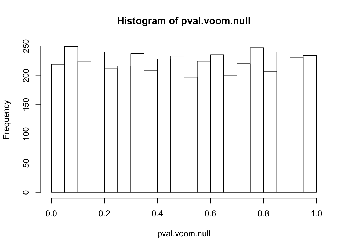
hist(pval.voom[data$null==1],25)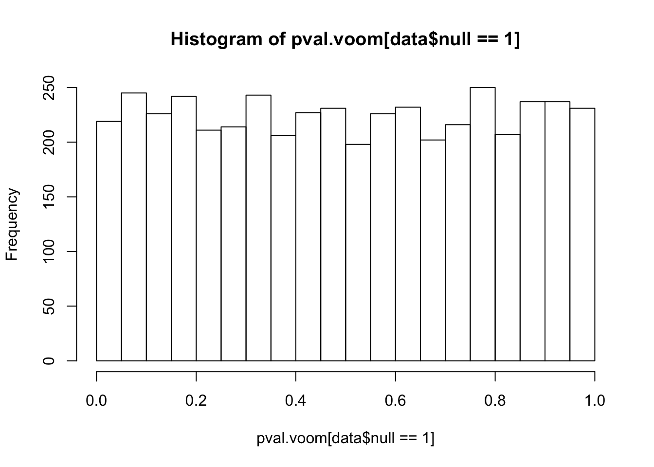
plot(voom$betahat[data$null==1],voom.null$betahat)
abline(0,1)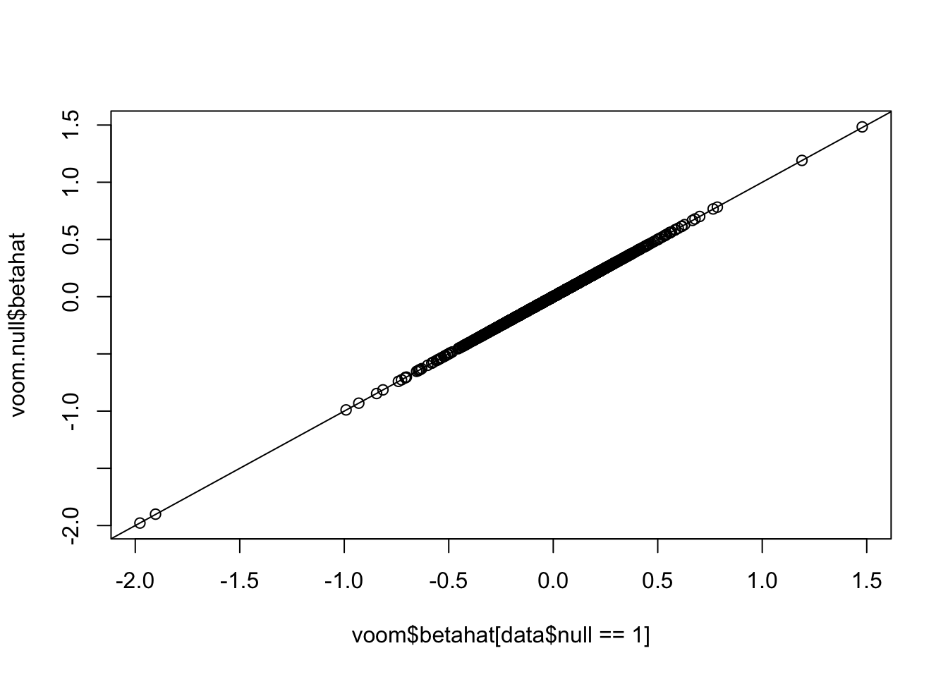
plot(voom$sebetahat[data$null==1],voom.null$sebetahat)
abline(0,1)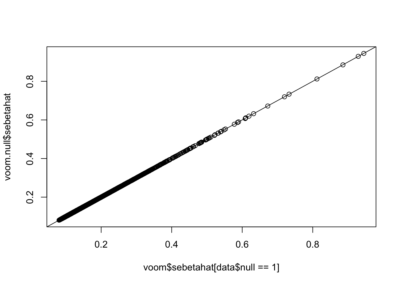
Estimate the null proportion from voom’s results by ash or qvalue: now it is closer to truth, suggesting that previous results in voom1.html are due to differences in library size. That is, the original simulation scheme was inducing effects in the “null” genes, and the method was detecting them - kind of correctly!
a.voom = ash(voom$betahat,voom$sebetahat,df=voom$df)
pi0.ash.voom = a.voom$fitted.g$pi[1]
pi0.ash.voom
[1] 0.8889627pi0.qval.voom = qvalue(pval.voom)$pi0
pi0.qval.voom[1] 0.9355572Try if log(counts+1)+OLS (David found it performed well in his simulations) or quantile normalization can fix this issue: log(counts+1)+OLS indeed gives uniform null p-values (which makes sense since it won’t introduce any extra correlation or inflation).
# log(counts+1)
logc = logc(data$counts, data$condition)
pval.logc = 2*(1-pt(abs(logc$betahat/logc$sebetahat),df=logc$df))

a.logc = ash(logc$betahat,logc$sebetahat,df=logc$df)
pi0.ash.logc = a.logc$fitted.g$pi[1]
pi0.ash.logc
[1] 0.8892937hist(pval.logc[data$null==1],25)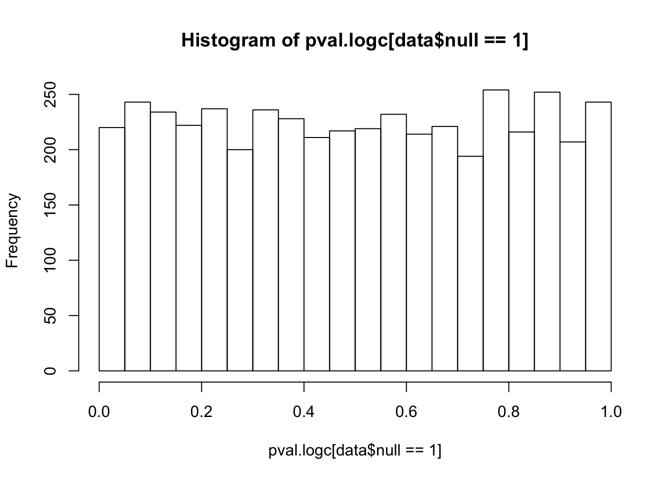
Session information
sessionInfo()R version 3.2.3 (2015-12-10)
Platform: x86_64-apple-darwin13.4.0 (64-bit)
Running under: OS X 10.11.2 (El Capitan)
locale:
[1] en_US.UTF-8/en_US.UTF-8/en_US.UTF-8/C/en_US.UTF-8/en_US.UTF-8
attached base packages:
[1] stats graphics grDevices utils datasets methods base
other attached packages:
[1] REBayes_0.61 Matrix_1.2-3 ashr_1.0.8 qvalue_2.0.0 edgeR_3.10.5
[6] limma_3.24.15 knitr_1.12.3
loaded via a namespace (and not attached):
[1] Rcpp_0.12.3 magrittr_1.5 MASS_7.3-45
[4] splines_3.2.3 pscl_1.4.9 munsell_0.4.2
[7] doParallel_1.0.10 lattice_0.20-33 SQUAREM_2014.8-1
[10] colorspace_1.2-6 foreach_1.4.3 stringr_1.0.0
[13] plyr_1.8.3 tools_3.2.3 parallel_3.2.3
[16] grid_3.2.3 gtable_0.1.2 iterators_1.0.8
[19] htmltools_0.3 assertthat_0.1 yaml_2.1.13
[22] digest_0.6.9 reshape2_1.4.1 ggplot2_2.0.0
[25] formatR_1.2.1 codetools_0.2-14 evaluate_0.8
[28] rmarkdown_0.9.2 stringi_1.0-1 Rmosek_7.1.2
[31] scales_0.3.0 truncnorm_1.0-7