Introduction to Mixture Models
Matt Bonakdarpour
2016-01-22
Last updated: 2019-03-31
Checks: 6 0
Knit directory: fiveMinuteStats/analysis/
This reproducible R Markdown analysis was created with workflowr (version 1.2.0). The Report tab describes the reproducibility checks that were applied when the results were created. The Past versions tab lists the development history.
Great! Since the R Markdown file has been committed to the Git repository, you know the exact version of the code that produced these results.
Great job! The global environment was empty. Objects defined in the global environment can affect the analysis in your R Markdown file in unknown ways. For reproduciblity it’s best to always run the code in an empty environment.
The command set.seed(12345) was run prior to running the code in the R Markdown file. Setting a seed ensures that any results that rely on randomness, e.g. subsampling or permutations, are reproducible.
Great job! Recording the operating system, R version, and package versions is critical for reproducibility.
Nice! There were no cached chunks for this analysis, so you can be confident that you successfully produced the results during this run.
Great! You are using Git for version control. Tracking code development and connecting the code version to the results is critical for reproducibility. The version displayed above was the version of the Git repository at the time these results were generated.
Note that you need to be careful to ensure that all relevant files for the analysis have been committed to Git prior to generating the results (you can use wflow_publish or wflow_git_commit). workflowr only checks the R Markdown file, but you know if there are other scripts or data files that it depends on. Below is the status of the Git repository when the results were generated:
Ignored files:
    Ignored:    .Rhistory
    Ignored:    .Rproj.user/
    Ignored:    analysis/.Rhistory
    Ignored:    analysis/bernoulli_poisson_process_cache/

Untracked files:
    Untracked:  _workflowr.yml
    Untracked:  analysis/CI.Rmd
    Untracked:  analysis/gibbs_structure.Rmd
    Untracked:  analysis/libs/
    Untracked:  analysis/results.Rmd
    Untracked:  analysis/shiny/tester/
    Untracked:  docs/MH_intro_files/
    Untracked:  docs/citations.bib
    Untracked:  docs/figure/MH_intro.Rmd/
    Untracked:  docs/figure/hmm.Rmd/
    Untracked:  docs/hmm_files/
    Untracked:  docs/libs/
    Untracked:  docs/shiny/tester/
Note that any generated files, e.g. HTML, png, CSS, etc., are not included in this status report because it is ok for generated content to have uncommitted changes.
These are the previous versions of the R Markdown and HTML files. If you’ve configured a remote Git repository (see ?wflow_git_remote), click on the hyperlinks in the table below to view them.
| File | Version | Author | Date | Message |
|---|---|---|---|---|
| html | 34bcc51 | John Blischak | 2017-03-06 | Build site. |
| Rmd | 5fbc8b5 | John Blischak | 2017-03-06 | Update workflowr project with wflow_update (version 0.4.0). |
| Rmd | 391ba3c | John Blischak | 2017-03-06 | Remove front and end matter of non-standard templates. |
| html | fb0f6e3 | stephens999 | 2017-03-03 | Merge pull request #33 from mdavy86/f/review |
| html | 0713277 | stephens999 | 2017-03-03 | Merge pull request #31 from mdavy86/f/review |
| Rmd | d674141 | Marcus Davy | 2017-02-27 | typos, refs |
| html | c3b365a | John Blischak | 2017-01-02 | Build site. |
| Rmd | 67a8575 | John Blischak | 2017-01-02 | Use external chunk to set knitr chunk options. |
| Rmd | 5ec12c7 | John Blischak | 2017-01-02 | Use session-info chunk. |
| Rmd | b94c4e9 | stephens999 | 2016-05-06 | minor edit |
| Rmd | bfd2478 | mbonakda | 2016-02-27 | update mixture model note |
| Rmd | 3bb3b73 | mbonakda | 2016-02-24 | add two mixture model vignettes + merge redundant info in markov chain vignettes |
Prerequisites
This document assumes basic familiarity with probability theory.
Overview
We often make simplifying modeling assumptions when analyzing a data set such as assuming each observation comes from one specific distribution (say, a Gaussian distribution). Then we proceed to estimate parameters of this distribution, like the mean and variance, using maximum likelihood estimation.
However, in many cases, assuming each sample comes from the same unimodal distribution is too restrictive and may not make intuitive sense. Often the data we are trying to model are more complex. For example, they might be multimodal – containing multiple regions with high probability mass. In this note, we describe mixture models which provide a principled approach to modeling such complex data.
Example 1
Suppose we are interested in simulating the price of a randomly chosen book. Since paperback books are typically cheaper than hardbacks, it might make sense to model the price of paperback books separately from hardback books. In this example, we will model the price of a book as a mixture model. We will have two mixture components in our model – one for paperback books, and one for hardbacks.
Let’s say that if we choose a book at random, there is a 50% chance of choosing a paperback and 50% of choosing hardback. These proportions are called mixture proportions. Assume the price of a paperback book is normally distributed with mean $9 and standard deviation $1 and the price of a hardback is normally distributed with a mean $20 and a standard deviation of $2. We could simulate book prices \(P_i\) in the following way:
- Sample \(Z_i \sim \text{Bernoulli}(0.5)\)
- If \(Z_i = 0\) draw \(P_i\) from the paperback distribution \(N(9,1)\). If \(Z_i = 1\), draw \(P_i\) from the hardback distribution \(N(20,2)\).
We implement this simulation in the code below:
NUM.SAMPLES <- 5000
prices      <- numeric(NUM.SAMPLES)
for(i in seq_len(NUM.SAMPLES)) {
  z.i <- rbinom(1,1,0.5)
  if(z.i == 0) prices[i] <- rnorm(1, mean = 9, sd = 1)
  else prices[i] <- rnorm(1, mean = 20, sd = 1)
}
hist(prices)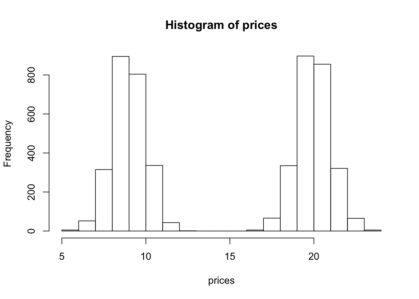
| Version | Author | Date |
|---|---|---|
| c3b365a | John Blischak | 2017-01-02 |
We see that our histogram is bimodal. Indeed, even though the mixture components are each normal distributions, the distribution of a randomly chosen book is not. We illustrate the true densities below: 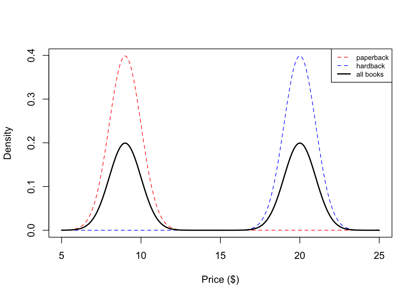
| Version | Author | Date |
|---|---|---|
| c3b365a | John Blischak | 2017-01-02 |
We see that the resulting probability density for all books is bimodal, and is therefore not normally distributed. In this example, we modeled the price of a book as a mixture of two components where each component was modeled as a Gaussian distribution. This is called a Gaussian mixture model (GMM).
Example 2
Now assume our data are the heights of students at the University of Chicago. Assume the height of a randomly chosen male is normally distributed with a mean equal to \(5'9\) and a standard deviation of \(2.5\) inches and the height of a randomly chosen female is \(N(5'4, 2.5)\). However, instead of 50/50 mixture proportions, assume that 75% of the population is female, and 25% is male. We simulate heights in a similar fashion as above, with the corresponding changes to the parameters:
NUM.SAMPLES <- 5000
heights      <- numeric(NUM.SAMPLES)
for(i in seq_len(NUM.SAMPLES)) {
  z.i <- rbinom(1,1,0.75)
  if(z.i == 0) heights[i] <- rnorm(1, mean = 69, sd = 2.5)
  else heights[i] <- rnorm(1, mean = 64, sd = 2.5)
}
hist(heights)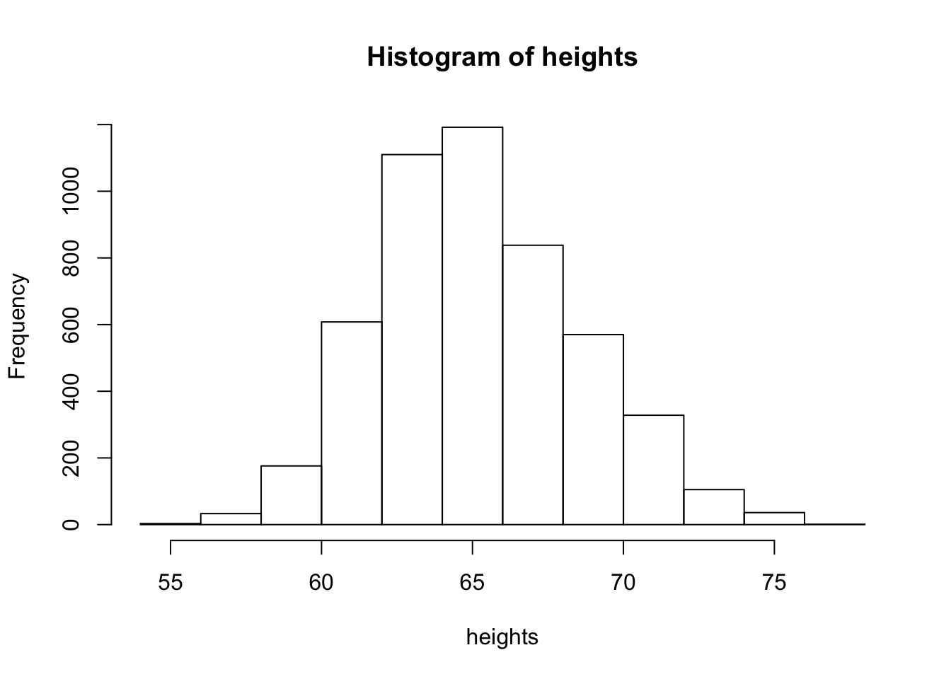
| Version | Author | Date |
|---|---|---|
| c3b365a | John Blischak | 2017-01-02 |
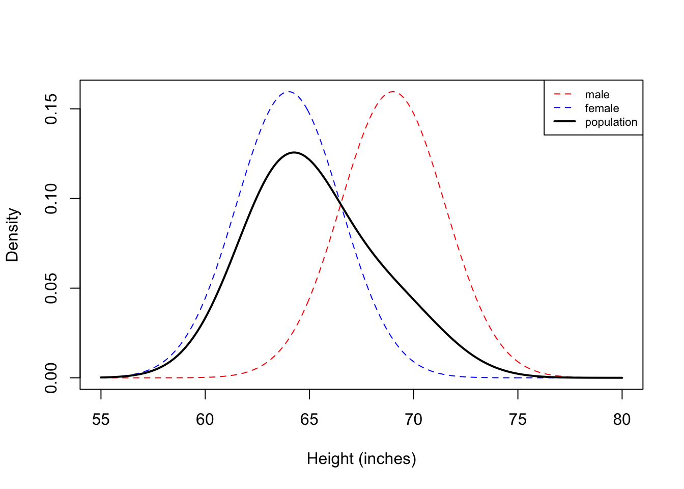
Now we see that histogram is unimodal. Are heights normally distributed under this model? We plot the corresponding densities below:
| Version | Author | Date |
|---|---|---|
| c3b365a | John Blischak | 2017-01-02 |
Here we see that the Gaussian mixture model is unimodal because there is so much overlap between the two densities. In this example, you can see that the population density is not symmetric, and therefore not normally distributed.
These two illustrative examples above give rise to the general notion of a mixture model which assumes each observation is generated from one of \(K\) mixture components. We formalize this notion in the next section.
Before moving on, we make one small pedagogical note that sometimes confuses students new to mixture models. You might recall that if \(X\) and \(Y\) are independent normal random variables, then \(Z=X+Y\) is also a normally distributed random variable. From this, you might wonder why the mixture models above aren’t normal. The reason is that \(X+Y\) is not a bivariate mixture of normals. It is a linear combination of normals. A random variable sampled from a simple Gaussian mixture model can be thought of as a two stage process. First, we randomly sample a component (e.g. male or female), then we sample our observation from the normal distribution corresponding to that component. This is clearly different than sampling \(X\) and \(Y\) from different normal distributions, then adding them together.
Definition
Assume we observe \(X_1,\ldots,X_n\) and that each \(X_i\) is sampled from one of \(K\) mixture components. In the second example above, the mixture components were \(\{\text{male,female}\}\). Associated with each random variable \(X_i\) is a label \(Z_i \in \{1,\ldots,K\}\) which indicates which component \(X_i\) came from. In our height example, \(Z_i\) would be either \(1\) or \(2\) depending on whether \(X_i\) was a male or female height. Often times we don’t observe \(Z_i\) (e.g. we might just obtain a list of heights with no gender information), so the \(Z_i\)’s are sometimes called latent variables.
From the law of total probability, we know that the marginal probability of \(X_i\) is: \[P(X_i = x) = \sum_{k=1}^K P(X_i=x|Z_i=k)\underbrace{P(Z_i=k)}_{\pi_k} = \sum_{k=1}^K P(X_i=x|Z_i=k)\pi_k\]
Here, the \(\pi_k\) are called mixture proportions or mixture weights and they represent the probability that \(X_i\) belongs to the \(k\)-th mixture component. The mixture proportions are nonnegative and they sum to one, \(\sum_{k=1}^K \pi_k = 1\). We call \(P(X_i|Z_i=k)\) the mixture component, and it represents the distribution of \(X_i\) assuming it came from component \(k\). The mixture components in our examples above were normal distributions.
For discrete random variables these mixture components can be any probability mass function \(p(. \mid Z_{k})\) and for continuous random variables they can be any probability density function \(f(. \mid Z_{k})\). The corresponding pmf and pdf for the mixture model is therefore:
\[p(x) = \sum_{k=1}^{K}\pi_k p(x \mid Z_{k})\] \[f_{x}(x) = \sum_{k=1}^{K}\pi_k f_{x \mid Z_{k}}(x \mid Z_{k}) \]
If we observe independent samples \(X_1,\ldots,X_n\) from this mixture, with mixture proportion vector \(\pi=(\pi_1, \pi_2,\ldots,\pi_K)\), then the likelihood function is: \[L(\pi) = \prod_{i=1}^n P(X_i|\pi) = \prod_{i=1}^n\sum_{k=1}^K P(X_i|Z_i=k)\pi_k\]
Now assume we are in the Gaussian mixture model setting where the \(k\)-th component is \(N(\mu_k, \sigma_k)\) and the mixture proportions are \(\pi_k\). A natural next question to ask is how to estimate the parameters \(\{\mu_k,\sigma_k,\pi_k\}\) from our observations \(X_1,\ldots,X_n\). We illustrate one approach in the introduction to EM vignette.
Acknowledgement: The “Examples” section above was taken from lecture notes written by Ramesh Sridharan.
sessionInfo()R version 3.5.2 (2018-12-20)
Platform: x86_64-apple-darwin15.6.0 (64-bit)
Running under: macOS Mojave 10.14.1
Matrix products: default
BLAS: /Library/Frameworks/R.framework/Versions/3.5/Resources/lib/libRblas.0.dylib
LAPACK: /Library/Frameworks/R.framework/Versions/3.5/Resources/lib/libRlapack.dylib
locale:
[1] en_US.UTF-8/en_US.UTF-8/en_US.UTF-8/C/en_US.UTF-8/en_US.UTF-8
attached base packages:
[1] stats graphics grDevices utils datasets methods base
loaded via a namespace (and not attached):
[1] workflowr_1.2.0 Rcpp_1.0.0 digest_0.6.18 rprojroot_1.3-2
[5] backports_1.1.3 git2r_0.24.0 magrittr_1.5 evaluate_0.12
[9] stringi_1.2.4 fs_1.2.6 whisker_0.3-2 rmarkdown_1.11
[13] tools_3.5.2 stringr_1.3.1 glue_1.3.0 xfun_0.4
[17] yaml_2.2.0 compiler_3.5.2 htmltools_0.3.6 knitr_1.21 This site was created with R Markdown