Mixture Models
Matthew Stephens
2021-01-25
Last updated: 2021-04-20
Checks: 7 0
Knit directory: fiveMinuteStats/analysis/
This reproducible R Markdown analysis was created with workflowr (version 1.6.2). The Checks tab describes the reproducibility checks that were applied when the results were created. The Past versions tab lists the development history.
Great! Since the R Markdown file has been committed to the Git repository, you know the exact version of the code that produced these results.
Great job! The global environment was empty. Objects defined in the global environment can affect the analysis in your R Markdown file in unknown ways. For reproduciblity it’s best to always run the code in an empty environment.
The command set.seed(12345) was run prior to running the code in the R Markdown file. Setting a seed ensures that any results that rely on randomness, e.g. subsampling or permutations, are reproducible.
Great job! Recording the operating system, R version, and package versions is critical for reproducibility.
Nice! There were no cached chunks for this analysis, so you can be confident that you successfully produced the results during this run.
Great job! Using relative paths to the files within your workflowr project makes it easier to run your code on other machines.
Great! You are using Git for version control. Tracking code development and connecting the code version to the results is critical for reproducibility.
The results in this page were generated with repository version cc566d3. See the Past versions tab to see a history of the changes made to the R Markdown and HTML files.
Note that you need to be careful to ensure that all relevant files for the analysis have been committed to Git prior to generating the results (you can use wflow_publish or wflow_git_commit). workflowr only checks the R Markdown file, but you know if there are other scripts or data files that it depends on. Below is the status of the Git repository when the results were generated:
Ignored files:
    Ignored:    .Rhistory
    Ignored:    .Rproj.user/
    Ignored:    analysis/.Rhistory
    Ignored:    analysis/bernoulli_poisson_process_cache/

Untracked files:
    Untracked:  _workflowr.yml
    Untracked:  analysis/CI.Rmd
    Untracked:  analysis/gibbs_structure.Rmd
    Untracked:  analysis/libs/
    Untracked:  analysis/results.Rmd
    Untracked:  analysis/shiny/tester/

Unstaged changes:
    Modified:   analysis/LR_and_BF.Rmd
    Modified:   analysis/MH-examples1.Rmd
    Modified:   analysis/MH_intro.Rmd
    Deleted:    analysis/r_simplemix_extended.Rmd
Note that any generated files, e.g. HTML, png, CSS, etc., are not included in this status report because it is ok for generated content to have uncommitted changes.
These are the previous versions of the repository in which changes were made to the R Markdown (analysis/mixture_models_01.Rmd) and HTML (docs/mixture_models_01.html) files. If you’ve configured a remote Git repository (see ?wflow_git_remote), click on the hyperlinks in the table below to view the files as they were in that past version.
| File | Version | Author | Date | Message |
|---|---|---|---|---|
| Rmd | cc566d3 | Matthew Stephens | 2021-04-20 | workflowr::wflow_publish(“analysis/mixture_models_01.Rmd”) |
| html | 4ced11a | Matthew Stephens | 2021-01-26 | Build site. |
| Rmd | 4b1238c | Matthew Stephens | 2021-01-26 | workflowr::wflow_publish(“mixture_models_01.Rmd”) |
| html | f4bada4 | Matthew Stephens | 2021-01-25 | Build site. |
| Rmd | be59a00 | Matthew Stephens | 2021-01-25 | workflowr::wflow_publish(“mixture_models_01.Rmd”) |
Pre-requisites
You should be familiar with basic probability, including the law of total probability, the notion of distibution and density, and with standard distributions (particularly the Gamma distribution).
Overview
This vignette introduces the idea of a mixture model. These models are widely used in statistics to model data where observations come from a “mixture” of two or more different distributions. The vignette introduces the basic idea of a mixture, its density/mass function, and terminology like “mixture proportions”, “mixture components” and “latent variable representation”.
Example
We begin this vignette with an example. A medical screening test for a disease involves measuring the concentration (\(X\)) of a protein in the blood. In normal individuals \(X\) has a Gamma distribution with mean 1 and shape 2 (so scale parameter is 0.5 as scale = mean/shape). In diseased individuals the protein becomes elevated, and \(X\) has a Gamma distribution with mean 2 and shape 2 (so scale =1).
Suppose that in a particular population 70% of individuals are normal and 30% are diseased. What will be the overall distribution of the protein levels in this population? How could you simulate from this distribution?
Answer
The overall distribution
Let \(X\) denote the protein concentration of a randomly chosen individual from the population. Let \(Z\) denote whether that same randomly-chosen individual is normal (\(Z=1\)) or diseased (\(Z=2\)). Here we assume that \(Z\) is unobserved; it has been introduced to help with notation and derivations.
By the law of total probability we can write the density of \(X\) as: \[p(x) = \Pr(Z = 1) p(x | Z=1) + \Pr(Z=2) p(x|Z=2).\] [In words, this represents $$p(x) = (normal) p(x | normal) + (diseased) p(x | diseased).]$$
From the information given we know that \(\Pr(\text{normal})=0.7\) and \(\Pr(\text{diseased})=0.3\). We also know \(p(x| \text{normal})\) and \(p(x| \text{diseased})\) are each given by the density of a gamma distribution. So we can write
\[p(x) = 0.7 \Gamma(x;0.5,2) + 0.3 \Gamma(x; 1, 2)\] where \(\Gamma(x; a,b)\) denotes the density of a Gamma distribution with scale \(a\) and shape \(b\).
This distribution is an example of a “mixture distribution” (in particular it is a “mixture of two Gamma distributions”). Here we plot the density of this mixture distribution (blue) as well as the densities of the individual distributions that were combined to make the mixture (black for normal, red for disease). In mixture terminology these individual distributions are called the “component distributions”.
x = seq(0,10,length=100)
plot(x, 0.7*dgamma(x,scale = 0.5,shape = 2) + 0.3 * dgamma(x,scale = 1,shape = 2)
       , col="blue", type="l", xlab="protein concentration", main="mixture distribution (blue)\n and component distributions (black,red)", ylab="density", ylim=c(0,0.8))
lines(x, dgamma(x,scale = 0.5,shape = 2), type="l", col="black")
lines(x, dgamma(x,scale = 1,shape = 2), type="l", col="red")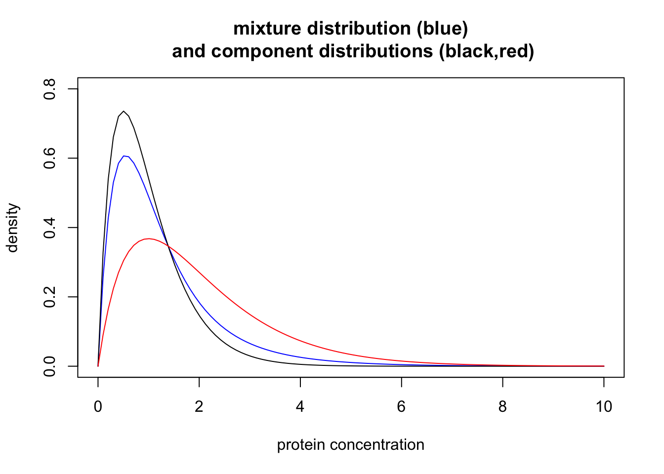
| Version | Author | Date |
|---|---|---|
| f4bada4 | Matthew Stephens | 2021-01-25 |
Simulation
One nice thing about mixture models is that they are super-easy to simulate from. The trick is to simulate both \((Z,X)\) from the joint distribution \(p(Z,X)\), and then to simply ignore \(Z\). This ensures that \(X\) comes from its marginal distribution \(p(X)\).
Simulating from \(p(Z,X)\) can be achieved by a two-stage process, simulating \(Z \sim p(Z)\) and then \(X|Z \sim p(X|Z)\), both of which are easy. The following code illustrates this idea by simulating 10000 samples from the mixture, and then plotting a histogram of the samples. As you can see the histogram closely matches the mixture density.
n = 10000 # number of samples
x = rep(0,n) # to store the samples
shape = c(2,2) # shapes of the two components
scale = c(0.5,1) # scales of the two components
for(i in 1:n){
  if(runif(1)<0.7)
    z=1 else z=2
  x[i] = rgamma(1,scale=scale[z],shape=shape[z])
}

# plot the histogram; note use of probability=TRUE so that it is scaled like a density (area=1). This makes it easy to compare with the theoretical density
hist(x,nclass=100,xlim=c(0,10),probability=TRUE)

# now plot density on top
xvec = seq(0,10,length=100)
lines(xvec, 0.7*dgamma(xvec,scale = 0.5,shape = 2) + 0.3 * dgamma(xvec,scale = 1,shape = 2))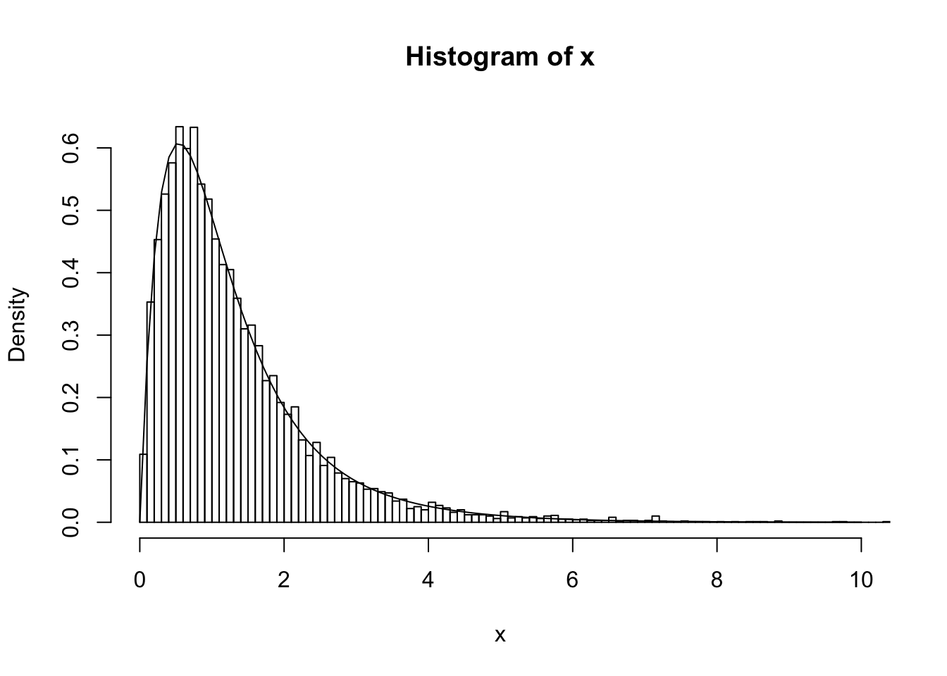
| Version | Author | Date |
|---|---|---|
| f4bada4 | Matthew Stephens | 2021-01-25 |
Exercises
The following exercises are designed to help you generalize the ideas used in example above to other settings.
1. Other mixture component distributions
In the above example there is nothing special about the Gamma distribution; one can similarly form mixtures of other distributions. This exercise illustrates this idea.
Consider modelling the heights of people sampled from a population that is 50% male and 50% female, where the males have heights that are normally distributed with mean 70 inches and standard deviation 3 inches, and the females have heights that are normally distributed with mean 64.5 inches and standard deviation 2.5 inches. Write the density of the mixture model. Identify the mixture proportions and the mixture component densities. Plot the mixture density and the component densities in a plot similar to the one in the example above.
2. More than two distributions
Similarly, there is nothing that limits us to mixing just two distributions – you can mix any number of distributions together. This exercise illustrates this idea.
Suppose that in the protein concentration example above the population consists of males and females, who have different rates of disease, and also different protein distributions. So now there are four different groups, “male, diseased”, “male, normal”, “female, diseased”, and “female, normal”. Making whatever assumptions you want about the component distributions (say what they are), and about the relative frequency of each group in the population (again, say what they are), write out a mixture distribution that could represent this situation. Plot the components of your assumed mixture and the mixture density.
3. Discrete data
The above example involves a mixture of two continuous distributions (Gamma distributions) and so the mixture distribution is also continuous. However, mixtures of discrete distributions work in the same way: you just use probability mass functions instead of probability density functions.
For example, let \(X\) denote the number of molecules of a particular gene in a cell randomly drawn from some population of cells. Assume that the population contains three cell types, in proportions \((0.2,0.4,0.4)\). Suppose that in each cell type the number of molecules follows a Poisson distribution with mean parameter \(\lambda=2,5,10\) respectively. The distribution of \(X\) is therefore a mixture of three poisson distributions. Can you write down its probability mass function?
General case
Putting the above ideas together we can write the density for a
mixture of \(K\) continuous distributions that have densities \(f_1,\dots,f_K\), in proportions \(\pi_1,\dots,\pi_K\). Such a mixture would have density: \[p(x) = \sum_{k=1}^K \pi_k f_k(x).\] (Exactly the same equation holds for a mixture of \(K\) discrete distibutions, but with \(p(x)\) and \(f_k\) representing probability mass functions instead of densities.)
Some important terminology:
This is called a mixture distribution (or mixture model, or just mixture) with \(K\) components. (Sometimes it is called a finite mixture because one can also further generalize the ideas to an uncountably infinite number of components!)
The \(f_1,\dots,f_K\) are called the component densities (or component distributions). So \(f_1\) is the density of component 1, and \(f_k\) is the density of component \(k\).
The \(\pi_1,\dots,\pi_K\) are called the mixture proportions. Of course we must have \(\pi_k \geq 0\) and \(\sum_{k=1}^K \pi_k =1\).
The unobserved random variable \(Z\) is sometimes referred to as the “component of origin” or the “component that gave rise to” the observation \(X\). If we have \(n\) observations \(X_1,\dots,X_n\) from a mixture model it is common to let \(Z_i\) denote the component that gave rise to \(X_i\).
Introducing unobserved variables, \(Z_i\), to help with computations or derivations is a common trick that is used beyond mixture models. This trick is sometimes called data augmentation. The unobserved random variables are sometimes called hidden variables or latent variables. Representing the mixture model \[p(x) = \sum_{k=1}^K \pi_k f_k(x).\] by the two-stage process: \[p(Z=k) = \pi_k\] \[p(x | Z=k) = f_k(x)\] is called the latent variable representation of the mixture model.
sessionInfo()R version 3.6.0 (2019-04-26)
Platform: x86_64-apple-darwin15.6.0 (64-bit)
Running under: macOS 10.16
Matrix products: default
BLAS: /Library/Frameworks/R.framework/Versions/3.6/Resources/lib/libRblas.0.dylib
LAPACK: /Library/Frameworks/R.framework/Versions/3.6/Resources/lib/libRlapack.dylib
locale:
[1] en_US.UTF-8/en_US.UTF-8/en_US.UTF-8/C/en_US.UTF-8/en_US.UTF-8
attached base packages:
[1] stats graphics grDevices utils datasets methods base
loaded via a namespace (and not attached):
[1] Rcpp_1.0.6 rstudioapi_0.13 whisker_0.4 knitr_1.29
[5] magrittr_1.5 workflowr_1.6.2 R6_2.4.1 rlang_0.4.10
[9] stringr_1.4.0 tools_3.6.0 xfun_0.16 git2r_0.27.1
[13] htmltools_0.5.0 ellipsis_0.3.1 yaml_2.2.1 digest_0.6.27
[17] rprojroot_1.3-2 tibble_3.0.4 lifecycle_1.0.0 crayon_1.3.4
[21] later_1.1.0.1 vctrs_0.3.4 fs_1.5.0 promises_1.1.1
[25] glue_1.4.2 evaluate_0.14 rmarkdown_2.3 stringi_1.4.6
[29] compiler_3.6.0 pillar_1.4.6 backports_1.1.10 httpuv_1.5.4
[33] pkgconfig_2.0.3 This site was created with R Markdown