Fit ebpmf on statisticalpaper abstracts (SLA) data
DongyueXie
2023-07-05
Last updated: 2023-07-09
Checks: 7 0
Knit directory: gsmash/
This reproducible R Markdown analysis was created with workflowr (version 1.6.2). The Checks tab describes the reproducibility checks that were applied when the results were created. The Past versions tab lists the development history.
Great! Since the R Markdown file has been committed to the Git repository, you know the exact version of the code that produced these results.
Great job! The global environment was empty. Objects defined in the global environment can affect the analysis in your R Markdown file in unknown ways. For reproduciblity it’s best to always run the code in an empty environment.
The command set.seed(20220606) was run prior to running
the code in the R Markdown file. Setting a seed ensures that any results
that rely on randomness, e.g. subsampling or permutations, are
reproducible.
Great job! Recording the operating system, R version, and package versions is critical for reproducibility.
Nice! There were no cached chunks for this analysis, so you can be confident that you successfully produced the results during this run.
Great job! Using relative paths to the files within your workflowr project makes it easier to run your code on other machines.
Great! You are using Git for version control. Tracking code development and connecting the code version to the results is critical for reproducibility.
The results in this page were generated with repository version 62315ed. See the Past versions tab to see a history of the changes made to the R Markdown and HTML files.
Note that you need to be careful to ensure that all relevant files for
the analysis have been committed to Git prior to generating the results
(you can use wflow_publish or
wflow_git_commit). workflowr only checks the R Markdown
file, but you know if there are other scripts or data files that it
depends on. Below is the status of the Git repository when the results
were generated:
Ignored files:
    Ignored:    .Rhistory
    Ignored:    .Rproj.user/
    Ignored:    analysis/figure/

Untracked files:
    Untracked:  chipexo_rep1_reverse.rds
    Untracked:  data/Citation.RData
    Untracked:  data/abstract.txt
    Untracked:  data/abstract.vocab.txt
    Untracked:  data/ap.txt
    Untracked:  data/ap.vocab.txt
    Untracked:  data/text.R
    Untracked:  data/tpm3.rds
    Untracked:  output/plots/
    Untracked:  output/tpm3_fit_fasttopics.rds
    Untracked:  output/tpm3_fit_stm.rds
    Untracked:  output/tpm3_fit_stm_slow.rds
    Untracked:  sla.rds

Unstaged changes:
    Modified:   analysis/PMF_splitting.Rmd
    Modified:   analysis/poisson_smoothing_benchmark.Rmd
Note that any generated files, e.g. HTML, png, CSS, etc., are not included in this status report because it is ok for generated content to have uncommitted changes.
These are the previous versions of the repository in which changes were
made to the R Markdown (analysis/fit_ebpmf_sla.Rmd) and
HTML (docs/fit_ebpmf_sla.html) files. If you’ve configured
a remote Git repository (see ?wflow_git_remote), click on
the hyperlinks in the table below to view the files as they were in that
past version.
| File | Version | Author | Date | Message |
|---|---|---|---|---|
| Rmd | 62315ed | DongyueXie | 2023-07-09 | wflow_publish("analysis/fit_ebpmf_sla.Rmd") |
Introduction
Dataset is from
library(flashier)Loading required package: magrittrdata <- read.table('data/abstract.txt')
data <- as.matrix(data)
vocab <- read.table('data/abstract.vocab.txt',colClasses = "character")[[1]]
# D_count is word by document matrix
D_count <- matrix(0,max(data[,2]),max(data[,1]))
for (t in 1:dim(data)[1]){
D_count[data[t,2], data[t,1]] <-data[t,3]
}
p <- dim(D_count)[1]
n <- dim(D_count)[2]
# Set some thresholds
w_num <- 3000 #number of words to keep
d_percent <- 0.6 #percentage of docs to keep
Mquantile <- 1 #Truncate quantile of M
#Only keep d_percent% longest documents
doc_count <- colSums(D_count)
doc_keep <- which(rank(-doc_count, ties.method = 'first')<=round(d_percent*n))
D_count <- D_count[,doc_keep]
#Only keep top w_num most frequent words
word_count <- rowSums(D_count)
word_keep <- which(rank(-word_count, ties.method = 'first')<=w_num)
D_count <- D_count[word_keep,]
vocab <- vocab[word_keep]
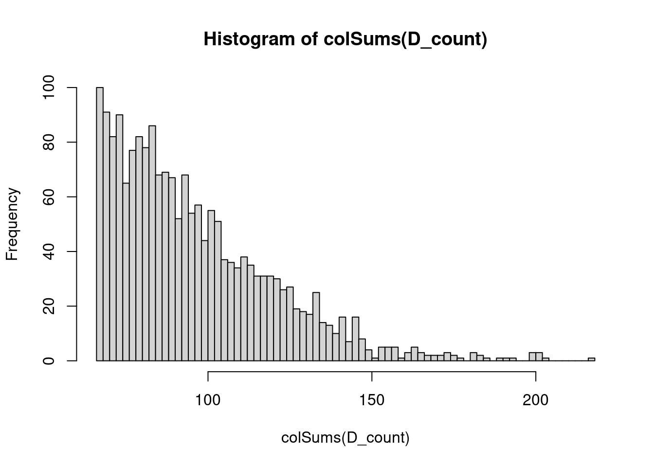
dim(D_count)[1] 2934 1916hist(colSums(D_count),breaks = 100)
## run ebpmf
library(ebpmf)
fit = ebpmf_log(t(D_count),flash_control=list(Kmax=10,
                                               ebnm.fn=c(ebnm::ebnm_point_exponential,ebnm::ebnm_point_exponential),
                                               loadings_sign=1,
                                               factors_sign = 1),
                var_type = 'by_col',
                init_control = list(init_tol=1e-4,single_gene_expmix=TRUE,deal_with_no_init_factor='...'),
                sigma2_control = list(return_sigma2_trace=T),
                general_control = list(maxiter=1,conv_tol=1e-5,save_init_val=TRUE,save_latent_M=T))
Initializing M...Solving VGA for column 1...100 ...200 ...300 ...400 ...500 ...600 ...700 ...800 ...900 ...1000 ...1100 ...1200 ...1300 ...1400 ...1500 ...1600 ...1700 ...1800 ...1900 ...2000 ...2100 ...2200 ...2300 ...2400 ...2500 ...2600 ...2700 ...2800 ...2900 ...
running initial flash fitWarning in scale.EF(EF): Fitting stopped after the initialization function
failed to find a non-zero factor.No structure found yet. Re-trying... 1
No structure found yet. Re-trying... 2
No structure found yet. Re-trying... 3
No structure found yet. Re-trying... 4
No structure found yet. Re-trying... 5
No structure found yet. Re-trying... 6
No structure found in default initialization.
Running iterations...Why no factor is added?
We see in the ebpmf fit that at the initialization, the model fails to find new factors, other than the intercepts.
We first extract the flash object, and reproduce the results.
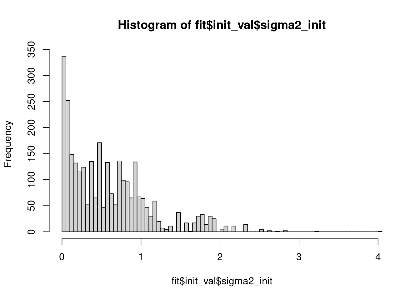
hist(fit$init_val$sigma2_init,breaks = 100)
range(fit$init_val$M_init)[1] -7.948548 2.544760# re-produce that flash could not add any more dimensions.
fit.flash = fit$fit_flash$flash.fit
fit.flash = flash.add.greedy(fit.flash, Kmax = 10,ebnm.fn = ebnm::ebnm_point_exponential,verbose = 1)Adding factor 3 to flash object...
Factor doesn't significantly increase objective and won't be added.
Wrapping up...
Done.How about just supply latent data to flash, and do not provide variances?
fit_flash = flash.init(fit$init_val$M_init,S=NULL,var.type = 2)
l0 = log(rowMeans(t(D_count)))
n = ncol(D_count)
p = nrow(D_count)
ebnm.fixed.l0 = function(x,s,g_init,fix_g,output){
    return(list(posterior=list(mean=l0,second_moment = l0^2),
                fitted_g = NULL,
                log_likelihood=sum(dnorm(x,l0,s,log=T))))
  }
fit_flash = flash.init.factors(fit_flash,list(cbind(l0), cbind(rep(1,p))),ebnm.fn = ebnm.fixed.l0) %>%
    flash.fix.factors(kset = 1, mode = 2)
f0 = log(cbind(colSums(t(D_count))/sum(exp(l0))))
  fit_flash = flash.init.factors(fit_flash,list(cbind(rep(1,n)), f0),ebnm.fn = ebnm::ebnm_normal) %>%
    flash.fix.factors(kset = 2, mode = 1)

fit_flash = flash.add.greedy(fit_flash, Kmax = 10,ebnm.fn = ebnm::ebnm_point_exponential)
Adding factor 3 to flash object...Warning in scale.EF(EF): Fitting stopped after the initialization function
failed to find a non-zero factor.Factor doesn't significantly increase objective and won't be added.
Wrapping up...
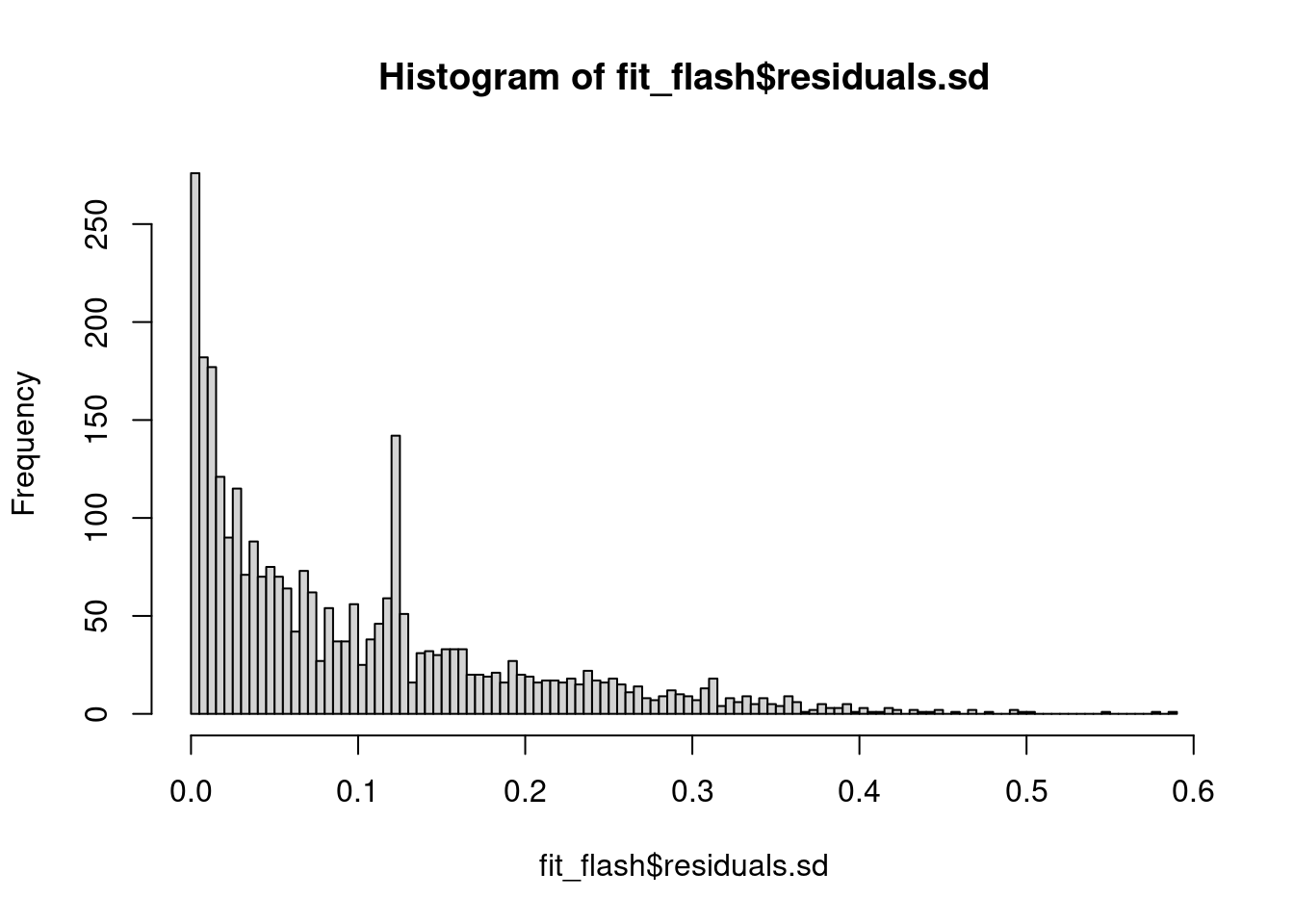
Done.hist(fit_flash$residuals.sd,breaks = 100)
Still not work. So maybe for this dataset, after accounting for the Document size and background word frequency, there’s no new multiplicative factor?
What if we subtract Document size and background word frequency from the latent data, and fit flash?
y = fit$init_val$M_init - tcrossprod(cbind(l0),cbind(rep(1,p))) - tcrossprod(cbind(rep(1,n)),cbind(f0))
res = flash(y,ebnm.fn = ebnm::ebnm_point_exponential,var.type = 2,backfit = T,greedy.Kmax = 10)
Adding factor 1 to flash object...Warning in scale.EF(EF): Fitting stopped after the initialization function
failed to find a non-zero factor.Factor doesn't significantly increase objective and won't be added.
Wrapping up...
Done.
No factors have been added. Skipping backfit.
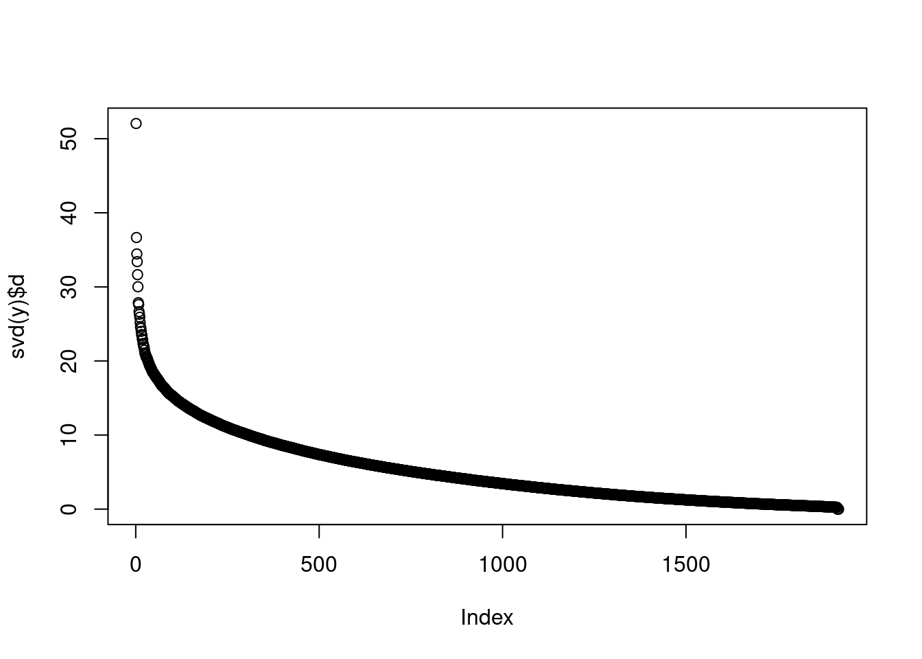
No factors have been added. Skipping nullcheck.plot(svd(y)$d)
sessionInfo()R version 4.1.0 (2021-05-18)
Platform: x86_64-pc-linux-gnu (64-bit)
Running under: CentOS Linux 7 (Core)
Matrix products: default
BLAS: /software/R-4.1.0-no-openblas-el7-x86_64/lib64/R/lib/libRblas.so
LAPACK: /software/R-4.1.0-no-openblas-el7-x86_64/lib64/R/lib/libRlapack.so
locale:
[1] LC_CTYPE=en_US.UTF-8 LC_NUMERIC=C LC_TIME=C
[4] LC_COLLATE=C LC_MONETARY=C LC_MESSAGES=C
[7] LC_PAPER=C LC_NAME=C LC_ADDRESS=C
[10] LC_TELEPHONE=C LC_MEASUREMENT=C LC_IDENTIFICATION=C
attached base packages:
[1] stats graphics grDevices utils datasets methods base
other attached packages:
[1] ebpmf_2.2.2 flashier_0.2.36 magrittr_2.0.3 workflowr_1.6.2
loaded via a namespace (and not attached):
[1] mcmc_0.9-7 bitops_1.0-7 matrixStats_0.59.0
[4] fs_1.5.0 progress_1.2.2 httr_1.4.5
[7] rprojroot_2.0.2 tools_4.1.0 bslib_0.4.2
[10] utf8_1.2.3 R6_2.5.1 irlba_2.3.5.1
[13] uwot_0.1.14 lazyeval_0.2.2 colorspace_2.1-0
[16] wavethresh_4.7.2 prettyunits_1.1.1 tidyselect_1.2.0
[19] ebpm_0.0.1.3 compiler_4.1.0 git2r_0.28.0
[22] glmnet_4.1-2 cli_3.6.1 quantreg_5.94
[25] SparseM_1.81 plotly_4.10.1 horseshoe_0.2.0
[28] sass_0.4.0 smashrgen_1.2.4 caTools_1.18.2
[31] scales_1.2.1 mvtnorm_1.1-2 SQUAREM_2021.1
[34] quadprog_1.5-8 pbapply_1.7-0 mixsqp_0.3-48
[37] stringr_1.5.0 digest_0.6.31 rmarkdown_2.9
[40] MCMCpack_1.6-3 deconvolveR_1.2-1 vebpm_0.4.8
[43] pkgconfig_2.0.3 htmltools_0.5.4 fastTopics_0.6-142
[46] highr_0.9 fastmap_1.1.0 invgamma_1.1
[49] htmlwidgets_1.6.1 rlang_1.1.1 rstudioapi_0.13
[52] shape_1.4.6 jquerylib_0.1.4 generics_0.1.3
[55] jsonlite_1.8.4 dplyr_1.1.0 smashr_1.3-6
[58] Matrix_1.5-3 Rcpp_1.0.10 munsell_0.5.0
[61] fansi_1.0.4 lifecycle_1.0.3 RcppZiggurat_0.1.6
[64] stringi_1.6.2 whisker_0.4 yaml_2.3.7
[67] MASS_7.3-54 Rtsne_0.16 grid_4.1.0
[70] parallel_4.1.0 promises_1.2.0.1 ggrepel_0.9.3
[73] crayon_1.5.2 lattice_0.20-44 cowplot_1.1.1
[76] splines_4.1.0 hms_1.1.2 knitr_1.33
[79] pillar_1.8.1 softImpute_1.4-1 codetools_0.2-18
[82] glue_1.6.2 evaluate_0.14 trust_0.1-8
[85] data.table_1.14.8 RcppParallel_5.1.7 foreach_1.5.1
[88] vctrs_0.6.2 nloptr_1.2.2.2 httpuv_1.6.1
[91] MatrixModels_0.5-1 gtable_0.3.1 purrr_1.0.1
[94] ebnm_1.0-11 tidyr_1.3.0 ashr_2.2-54
[97] cachem_1.0.5 ggplot2_3.4.1 xfun_0.24
[100] Rfast_2.0.7 coda_0.19-4 later_1.3.0
[103] mr.ash_0.1-87 survival_3.2-11 viridisLite_0.4.1
[106] truncnorm_1.0-8 tibble_3.2.1 iterators_1.0.13
[109] ellipsis_0.3.2