multiplicative vs additive PMF
DongyueXie
2023-08-17
Last updated: 2023-09-12
Checks: 7 0
Knit directory: gsmash/
This reproducible R Markdown analysis was created with workflowr (version 1.6.2). The Checks tab describes the reproducibility checks that were applied when the results were created. The Past versions tab lists the development history.
Great! Since the R Markdown file has been committed to the Git repository, you know the exact version of the code that produced these results.
Great job! The global environment was empty. Objects defined in the global environment can affect the analysis in your R Markdown file in unknown ways. For reproduciblity it’s best to always run the code in an empty environment.
The command set.seed(20220606) was run prior to running
the code in the R Markdown file. Setting a seed ensures that any results
that rely on randomness, e.g. subsampling or permutations, are
reproducible.
Great job! Recording the operating system, R version, and package versions is critical for reproducibility.
Nice! There were no cached chunks for this analysis, so you can be confident that you successfully produced the results during this run.
Great job! Using relative paths to the files within your workflowr project makes it easier to run your code on other machines.
Great! You are using Git for version control. Tracking code development and connecting the code version to the results is critical for reproducibility.
The results in this page were generated with repository version 7be2eae. See the Past versions tab to see a history of the changes made to the R Markdown and HTML files.
Note that you need to be careful to ensure that all relevant files for
the analysis have been committed to Git prior to generating the results
(you can use wflow_publish or
wflow_git_commit). workflowr only checks the R Markdown
file, but you know if there are other scripts or data files that it
depends on. Below is the status of the Git repository when the results
were generated:
Ignored files:
    Ignored:    .Rhistory
    Ignored:    .Rproj.user/

Untracked files:
    Untracked:  analysis/GO_ORA_montoro.Rmd
    Untracked:  analysis/GO_ORA_pbmc_purified.Rmd
    Untracked:  analysis/fit_ebpmf_sla_2000.Rmd
    Untracked:  analysis/poisson_deviance.Rmd
    Untracked:  analysis/sla_data.Rmd
    Untracked:  chipexo_rep1_reverse.rds
    Untracked:  data/Citation.RData
    Untracked:  data/SLA/
    Untracked:  data/abstract.txt
    Untracked:  data/abstract.vocab.txt
    Untracked:  data/ap.txt
    Untracked:  data/ap.vocab.txt
    Untracked:  data/sla_2000.rds
    Untracked:  data/sla_full.rds
    Untracked:  data/text.R
    Untracked:  data/tpm3.rds
    Untracked:  output/driving_gene_pbmc.rds
    Untracked:  output/pbmc_gsea.rds
    Untracked:  output/plots/
    Untracked:  output/tpm3_fit_fasttopics.rds
    Untracked:  output/tpm3_fit_stm.rds
    Untracked:  output/tpm3_fit_stm_slow.rds
    Untracked:  sla.rds

Unstaged changes:
    Modified:   analysis/PMF_splitting.Rmd
    Modified:   analysis/fit_ebpmf_sla.Rmd
    Modified:   analysis/index.Rmd
    Modified:   code/poisson_STM/structure_plot.R
    Modified:   code/poisson_mean/pois_log_normal_mle.R
Note that any generated files, e.g. HTML, png, CSS, etc., are not included in this status report because it is ok for generated content to have uncommitted changes.
These are the previous versions of the repository in which changes were
made to the R Markdown
(analysis/multiplicative_additive.Rmd) and HTML
(docs/multiplicative_additive.html) files. If you’ve
configured a remote Git repository (see ?wflow_git_remote),
click on the hyperlinks in the table below to view the files as they
were in that past version.
| File | Version | Author | Date | Message |
|---|---|---|---|---|
| Rmd | 7be2eae | DongyueXie | 2023-09-12 | wflow_publish("analysis/multiplicative_additive.Rmd") |
Introduction
I want to find a simple example to illustrate the difference between multiplicative and additive methods.
The multiplicative effects come with the log link in Poisson model can be understood as follows:
Let \(\boldsymbol{x}_i\) denote the a data vector, then we can write \(\mathbb{E}(\boldsymbol{x}_i) = \exp(\boldsymbol{\mu} + \sum_kl_{ik}\boldsymbol{f}_k)=\exp(\boldsymbol{\mu})\prod_k \exp(l_{ik}\boldsymbol{f}_k).\)
Here I start with a very simple example where the two factors look like:
\(\boldsymbol{f}_1 = (1,1,1,1,0,0,0,0), \boldsymbol{f}_2=(1,1,0,0,1,1,0,0)\).
So for the \(i\)th sample, its mean is \(background\times \exp(l_{i1}\boldsymbol{f}_1)\times \exp(l_{i2}\boldsymbol{f}_2)\).
WLOG let’s set background to be all 1’s. The observations(elements) of \(i\)th sample would be \(\exp(l_{i1})\exp(l_{i2}),\exp(l_{i1}),\exp(l_{i2}),1\).
Let’s set the following loadings:
- \(l_1=l_2=0\); 2. \(l_1=2, l_2=0\); 3. \(l_1=0,l_2=2\); 4. \(l_1=4,l_2=2\).
The corresponding Poisson rates are
\((1,1,1,1),(\exp(2),\exp(2),1,1),(\exp(2),1,\exp(2),1), (\exp(6),\exp(4),\exp(2),1)\).
N = 100
Ftrue = cbind(c(1,1,1,1,0,0,0,0),c(1,1,0,0,1,1,0,0))
set.seed(12345)
#Ltrue = matrix(rexp(N*2,1),nrow=N)
Ltrue = cbind(rep(c(0,2,0,4),each=N/4),rep(c(0,0,2,2),each=N/4))
mu = tcrossprod(Ltrue,Ftrue)
lambda = exp(mu)
Y = matrix(rpois(N*nrow(Ftrue),lambda),nrow=N)

Ftrue
[,1] [,2]
[1,] 1 1
[2,] 1 1
[3,] 1 0
[4,] 1 0
[5,] 0 1
[6,] 0 1
[7,] 0 0
[8,] 0 0plot(Ltrue[,1])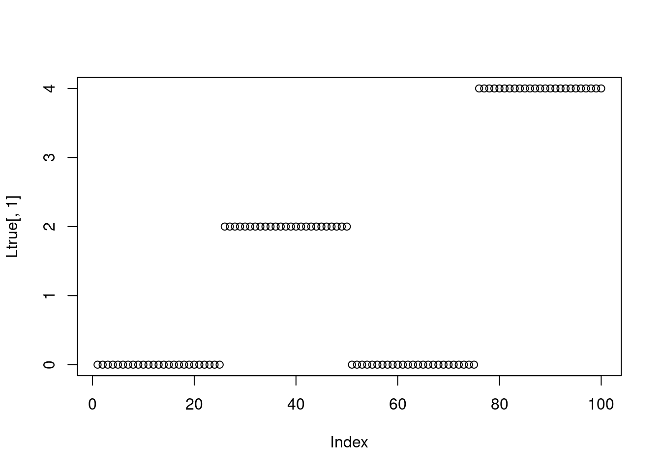
plot(Ltrue[,2])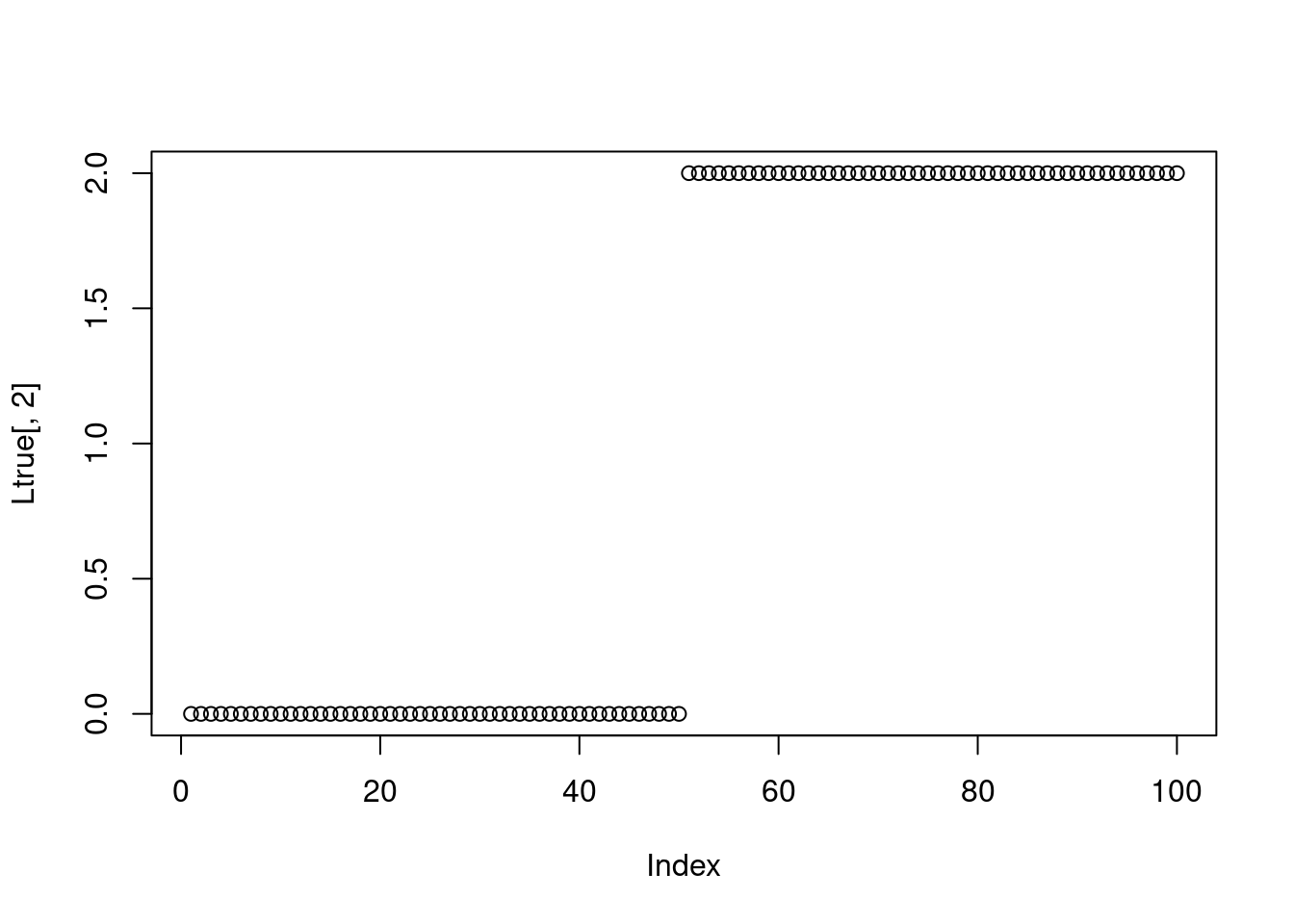
Can NMF recover Ltrue and Ftrue, if we directly apply NMF on \(LF\)?
nmf_fit = NNLM::nnmf(mu,k=2,loss='mse')
plot(nmf_fit$H[1,])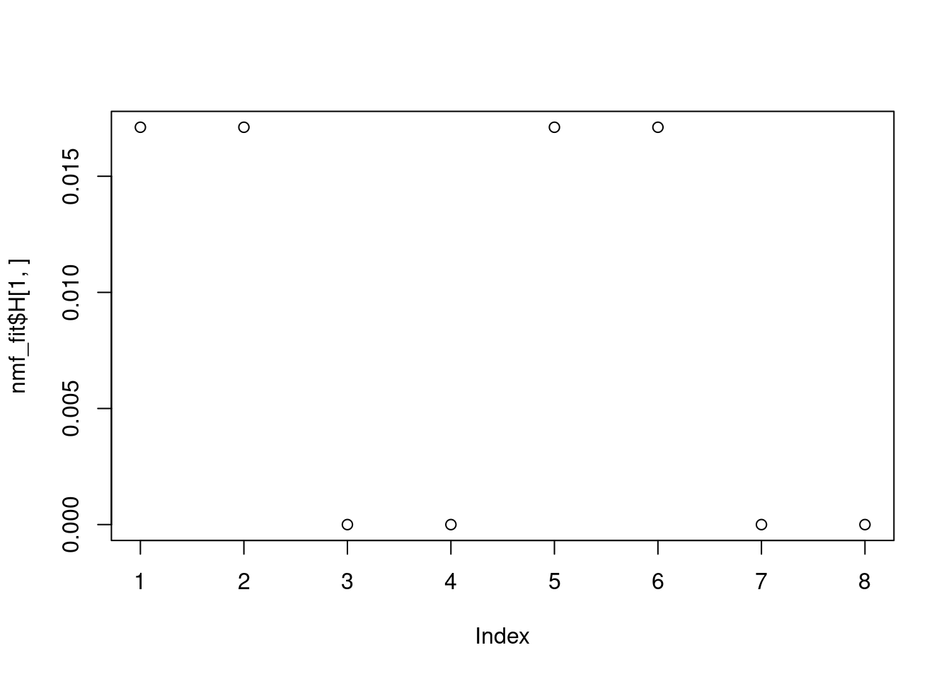
plot(nmf_fit$H[2,])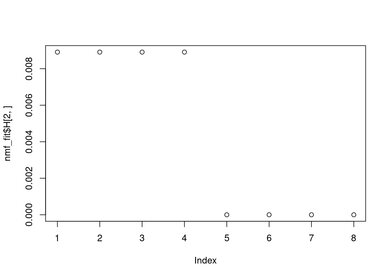
Looks good.
How about running EBNMF on \(LF\)? It is not working because “The data matrix must not have any rows or columns whose entries are either identically zero or all missing.”
ebnmf_fit = flashier::flash(mu,ebnm_fn = c(ebnm::ebnm_unimodal_nonnegative,ebnm::ebnm_unimodal_nonnegative),var_type = 0,backfit = T)Now we fit NMF to the data matrix Y:
Let’s start with k=2
fit0 = fastTopics::fit_poisson_nmf(Y,2)Initializing factors using Topic SCORE algorithm.
Initializing loadings by running 10 SCD updates.
Fitting rank-2 Poisson NMF to 100 x 8 dense matrix.
Running 100 SCD updates, without extrapolation (fastTopics 0.6-142).plot(fit0$F[,1])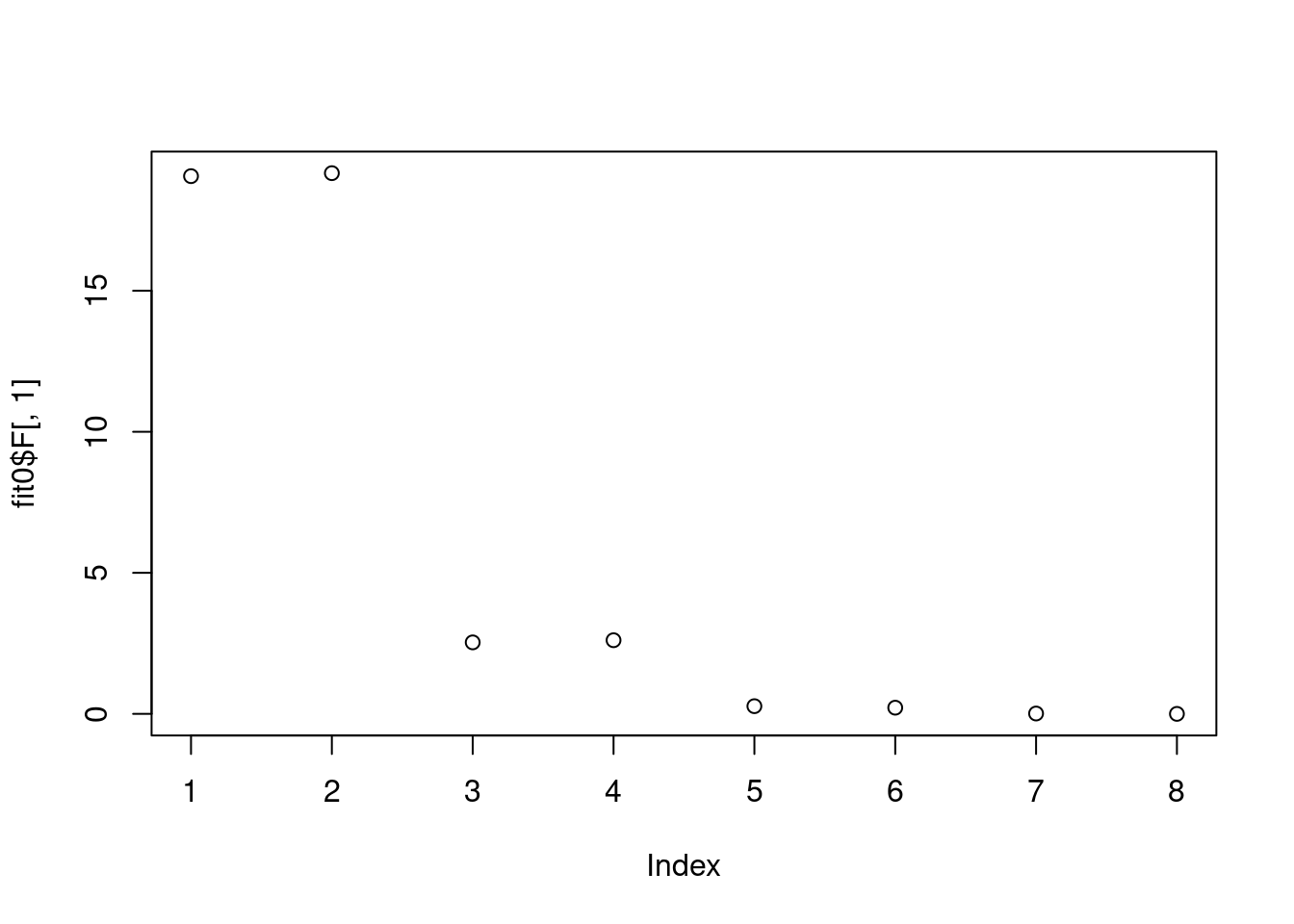
plot(fit0$F[,2])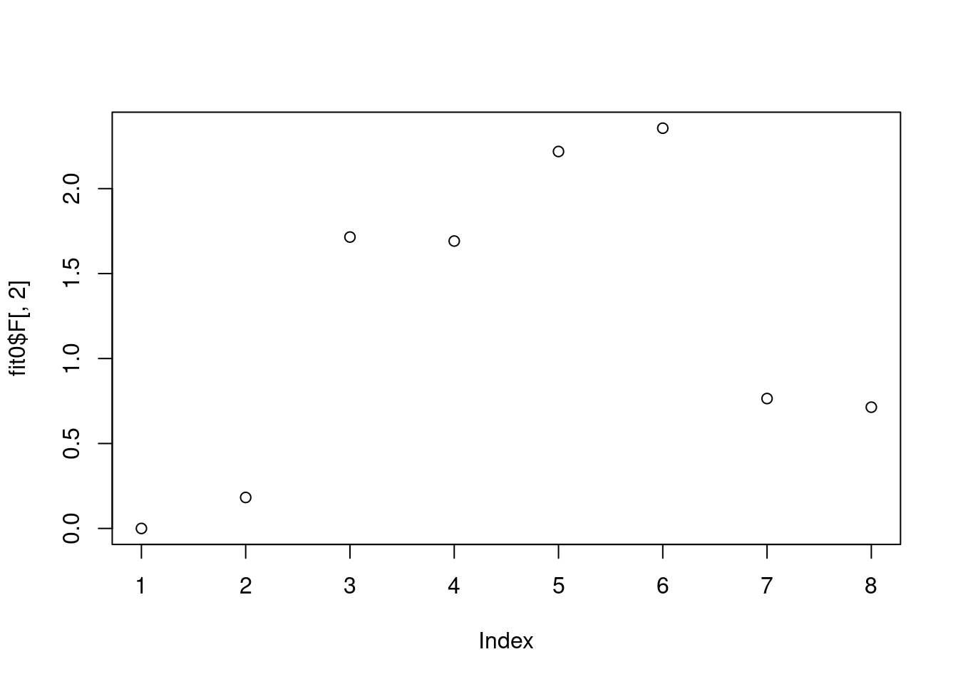
plot(fit0$L[,1])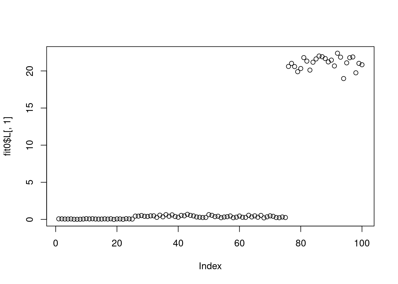
plot(fit0$L[,2])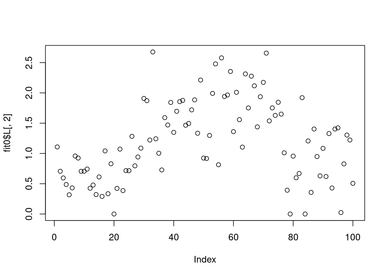
Then k = 3
fit0 = fastTopics::fit_poisson_nmf(Y,3)Initializing factors using Topic SCORE algorithm.Warning in value[[3L]](cond): Topic SCORE failure occurred; falling back to
init.method == "random"Topic SCORE failure occurred; using random initialization instead.
Fitting rank-3 Poisson NMF to 100 x 8 dense matrix.
Running 100 SCD updates, without extrapolation (fastTopics 0.6-142).plot(fit0$F[,1])
plot(fit0$F[,2])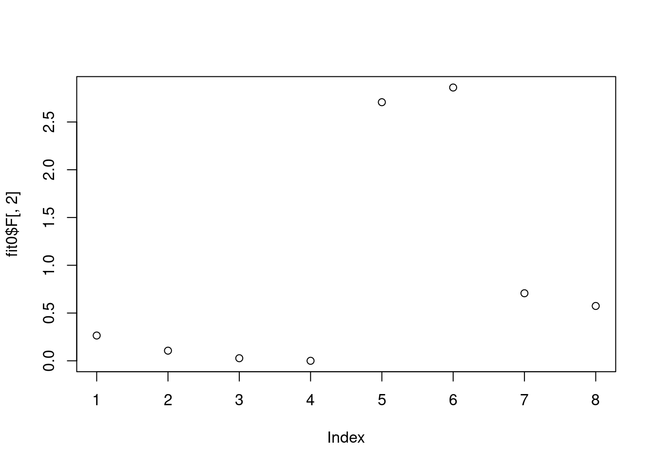
plot(fit0$F[,3])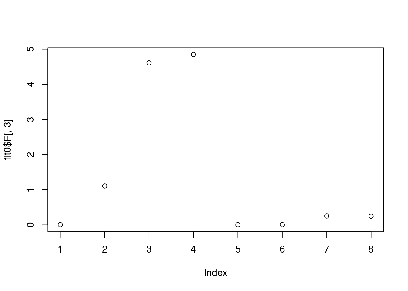
plot(fit0$L[,1])
plot(fit0$L[,2])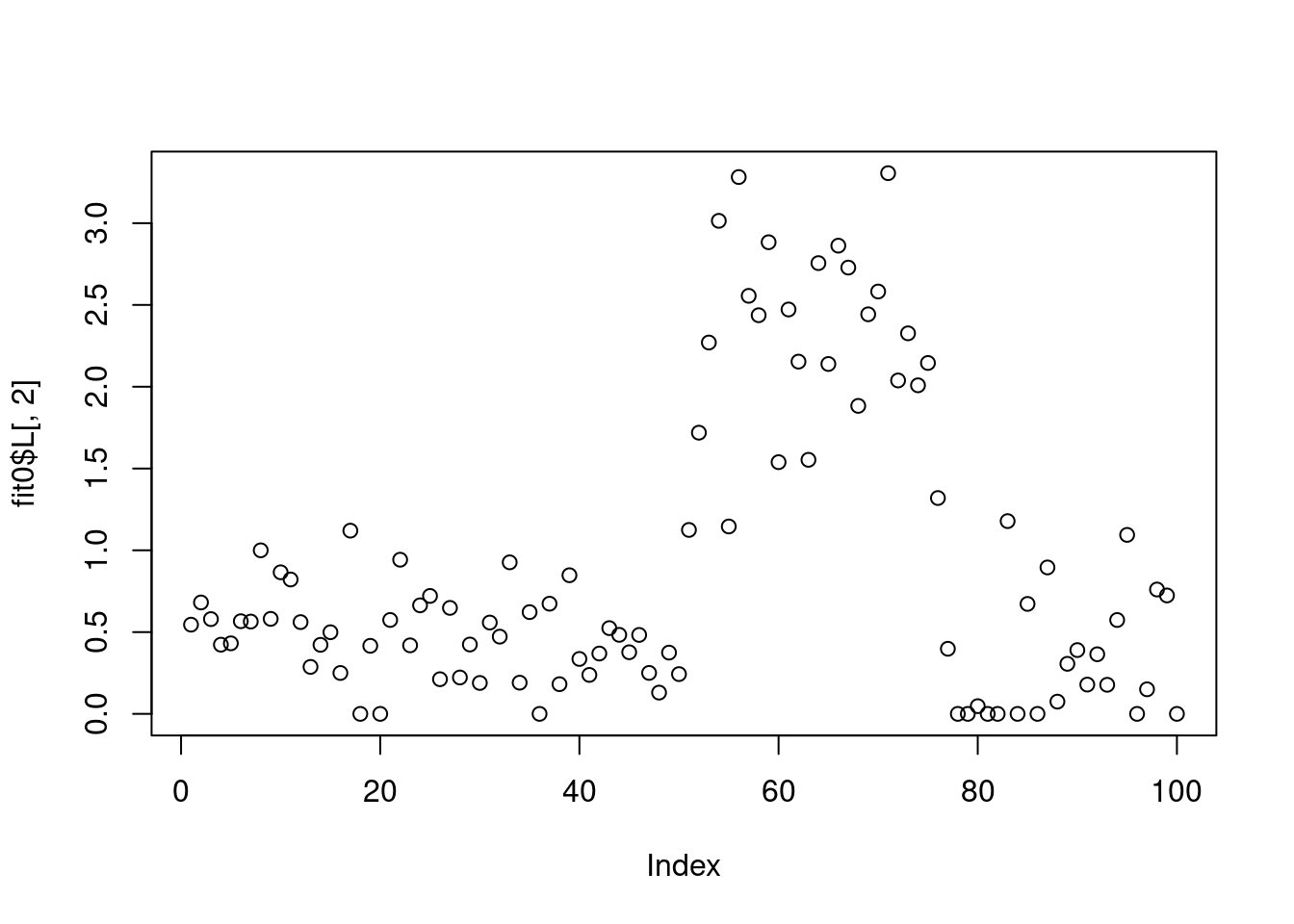
plot(fit0$L[,3])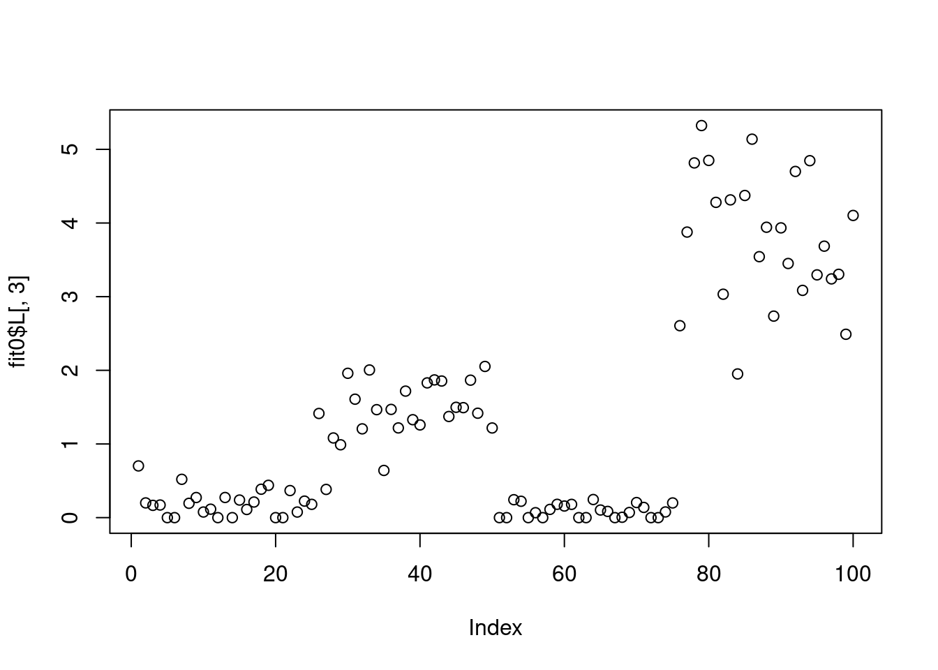
Now we try to fit ebnmf on log transformed data:
fit2 = flashier::flash(log(1+Y),ebnm_fn = c(ebnm::ebnm_point_exponential,ebnm::ebnm_point_exponential),var_type = 0,backfit = T)Adding factor 1 to flash object...
Adding factor 2 to flash object...
Adding factor 3 to flash object...
Adding factor 4 to flash object...
Factor doesn't significantly increase objective and won't be added.
Wrapping up...
Done.
Backfitting 3 factors (tolerance: 1.19e-05)...
Difference between iterations is within 1.0e+01...
Difference between iterations is within 1.0e+00...
Difference between iterations is within 1.0e-01...
Difference between iterations is within 1.0e-02...
Difference between iterations is within 1.0e-03...
Difference between iterations is within 1.0e-04...
Difference between iterations is within 1.0e-05...
Wrapping up...
Done.
Nullchecking 3 factors...
Done.plot(fit2$F_pm[,1])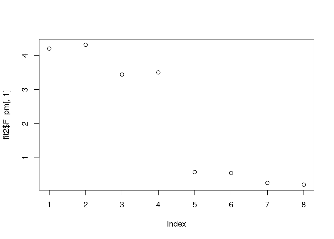
plot(fit2$F_pm[,2])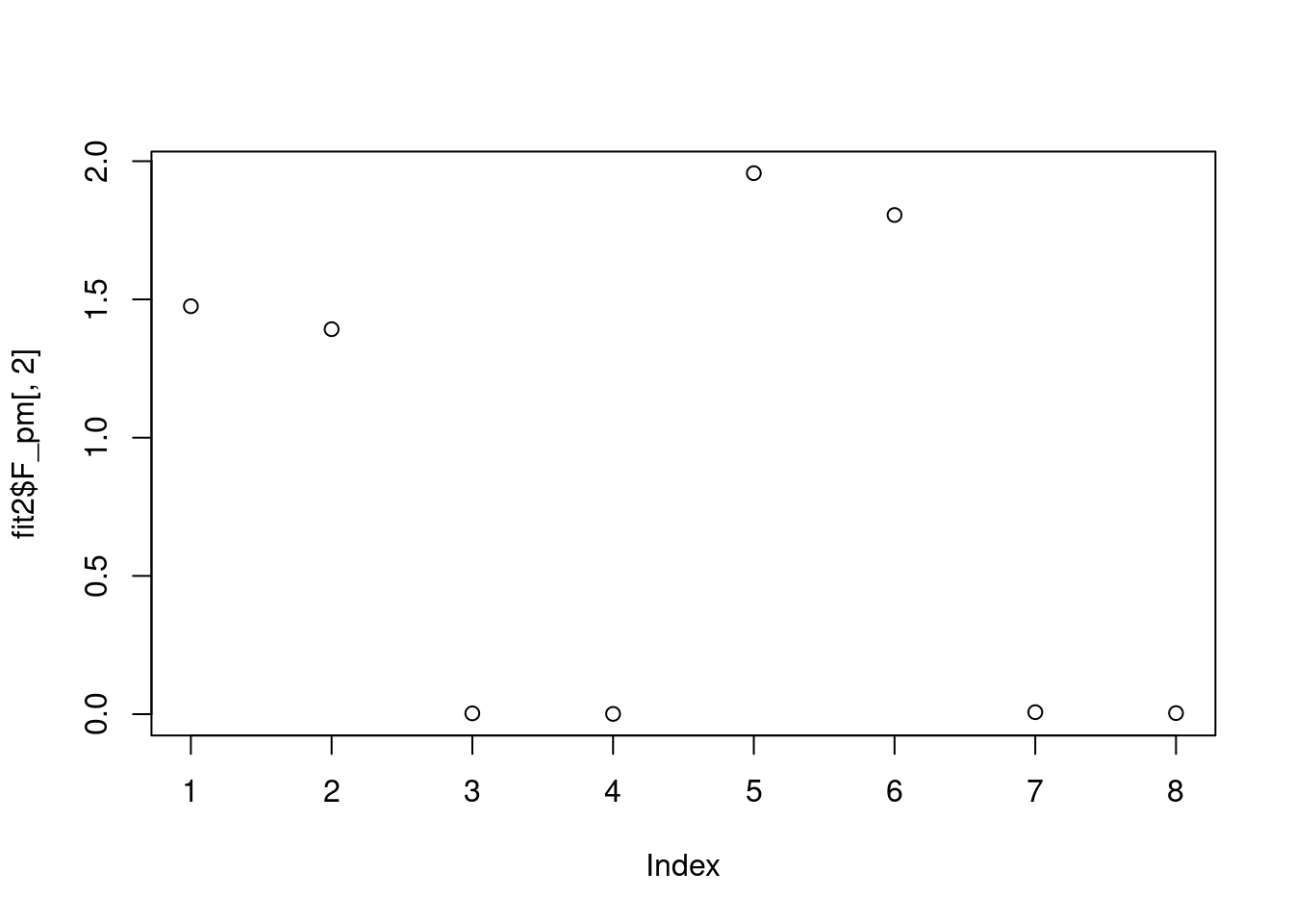
plot(fit2$F_pm[,3])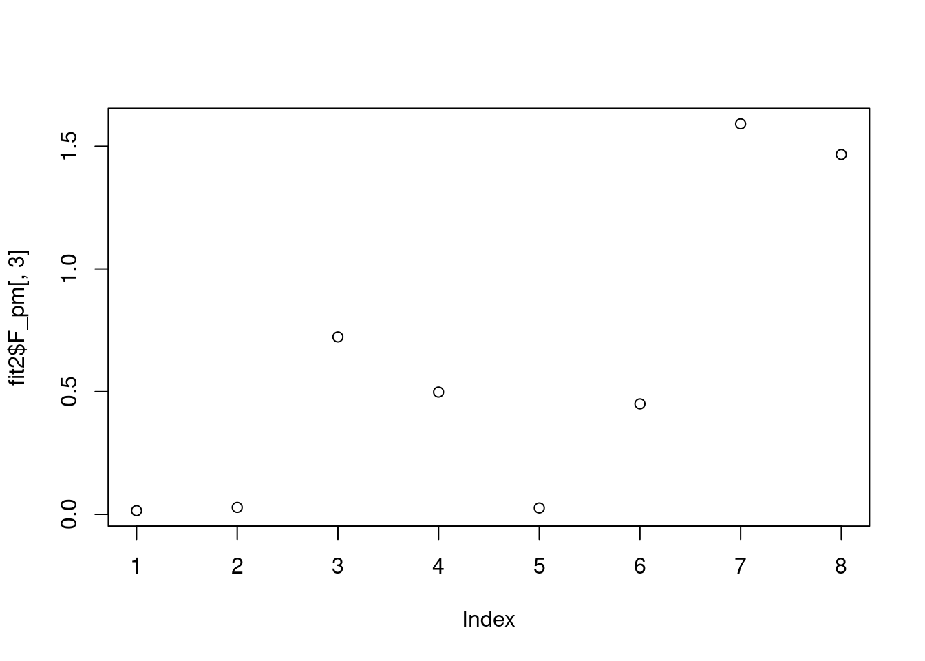
plot(fit2$L_pm[,1])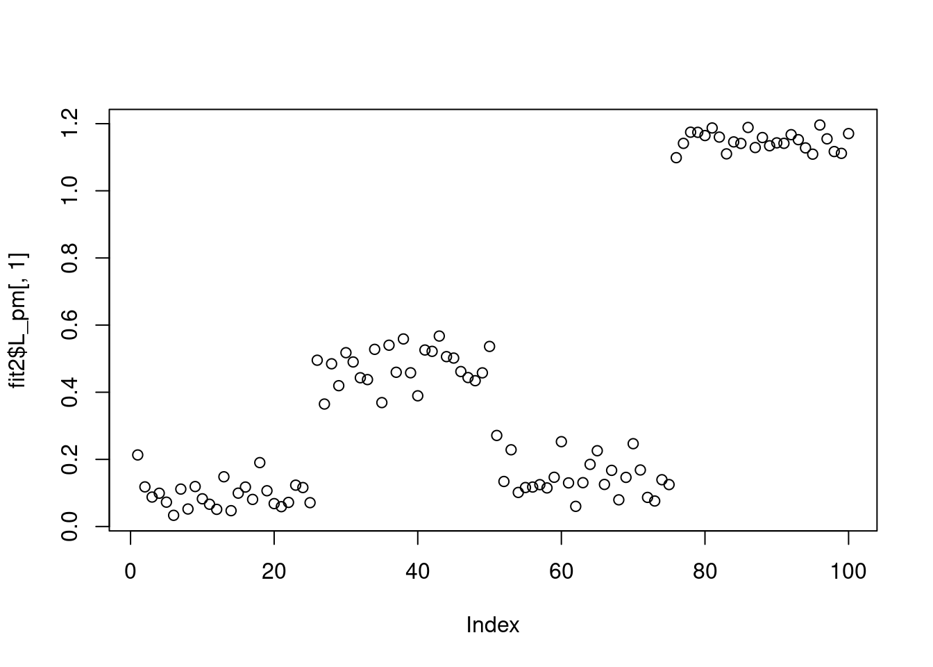
plot(fit2$L_pm[,2])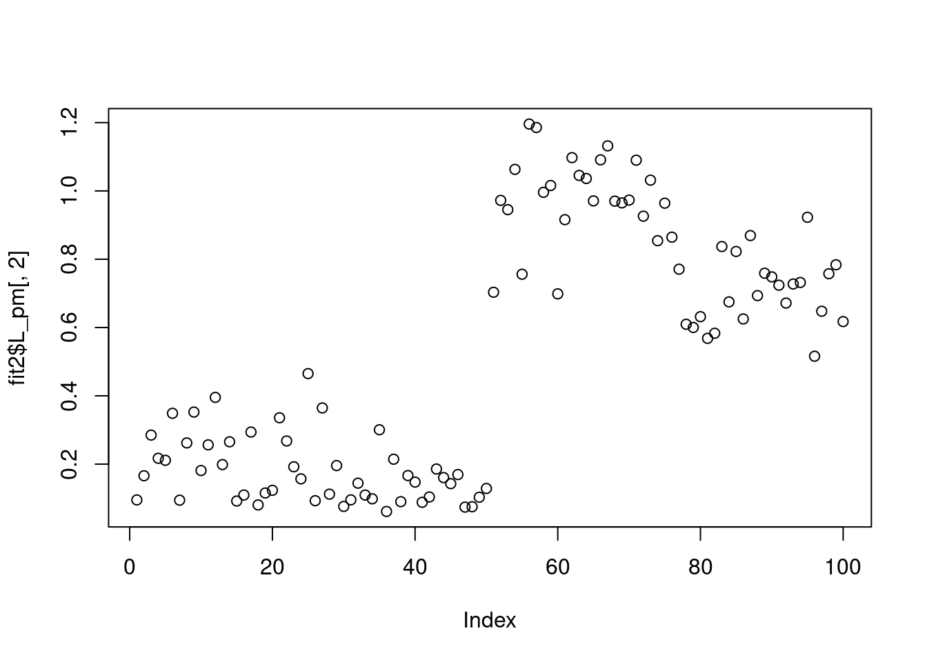
plot(fit2$L_pm[,3])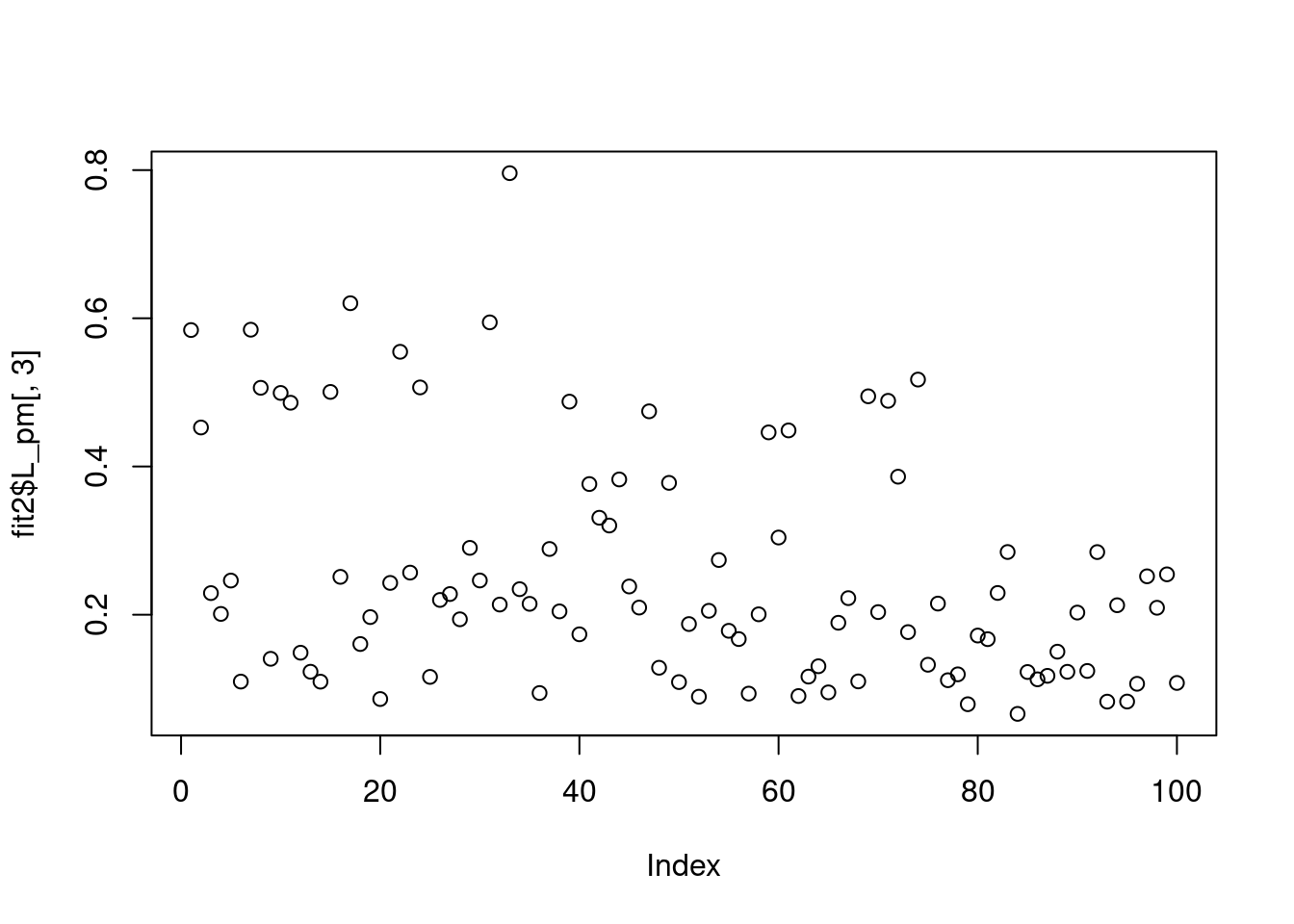
fit2 = flashier::flash(log(0.5+Y),ebnm_fn = c(ebnm::ebnm_point_exponential,ebnm::ebnm_point_exponential),var_type = 0,backfit = T)Adding factor 1 to flash object...
Adding factor 2 to flash object...
Adding factor 3 to flash object...
Factor doesn't significantly increase objective and won't be added.
Wrapping up...
Done.
Backfitting 2 factors (tolerance: 1.19e-05)...
Difference between iterations is within 1.0e+01...
Difference between iterations is within 1.0e+00...
Difference between iterations is within 1.0e-01...
Difference between iterations is within 1.0e-02...
Difference between iterations is within 1.0e-03...
Difference between iterations is within 1.0e-04...
Difference between iterations is within 1.0e-05...
Wrapping up...
Done.
Nullchecking 2 factors...
Done.plot(fit2$F_pm[,1])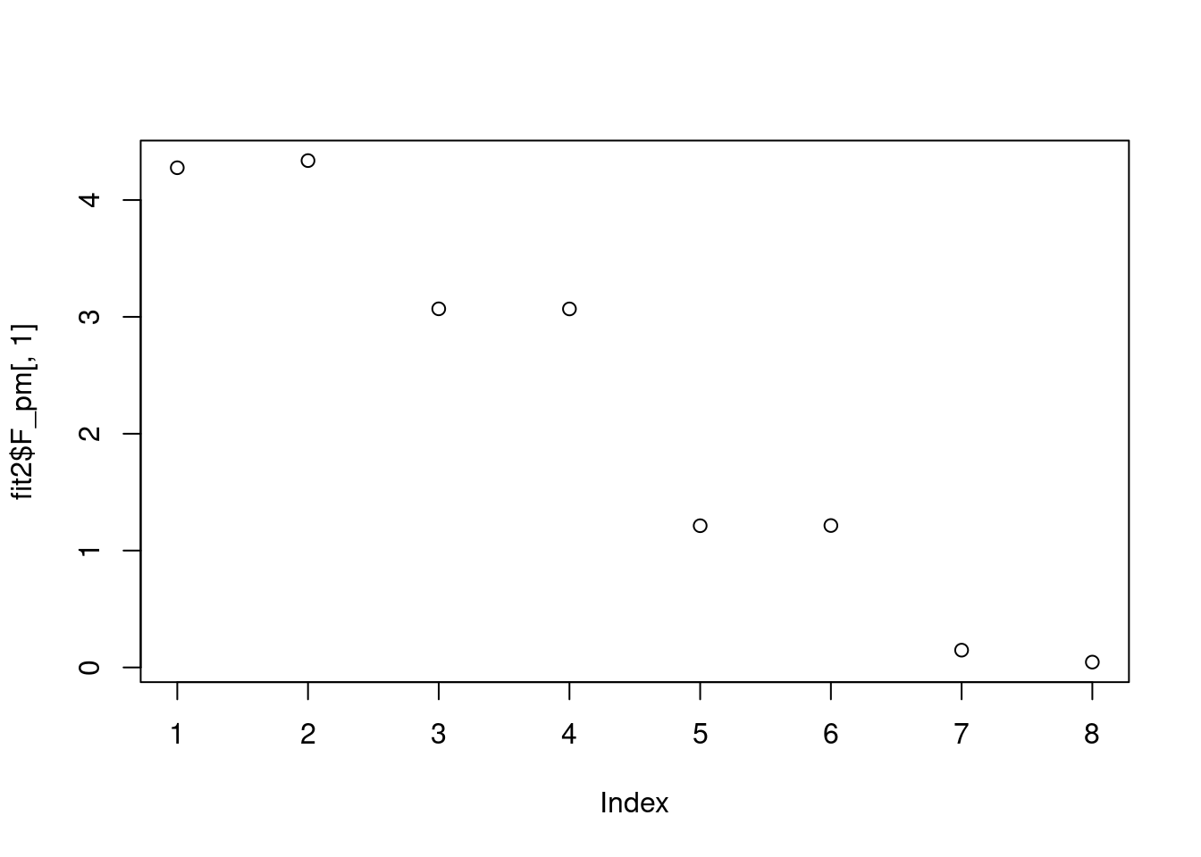
plot(fit2$F_pm[,2])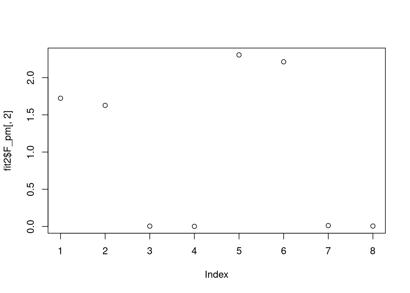
fit1 = ebpmf::ebpmf_log(Y,l0=0,f0=0,var_type = 'constant',
                        flash_control = list(fix_l0=T,fix_f0=T,ebnm.fn=c(ebnm::ebnm_unimodal_nonnegative,ebnm::ebnm_unimodal_nonnegative),
                                                                         loadings_sign=1,factors_sign =1))
Initializing
Solving VGA constant...For large matrix this may require large memory usage
Running initial EBMF fit
Running iterations...
iter 10, avg elbo=-2.6956, K=4
iter 20, avg elbo=-2.65927, K=4
iter 30, avg elbo=-2.6475, K=4
iter 40, avg elbo=-2.63747, K=4
iter 50, avg elbo=-2.62896, K=4
sessionInfo()R version 4.1.0 (2021-05-18)
Platform: x86_64-pc-linux-gnu (64-bit)
Running under: CentOS Linux 7 (Core)
Matrix products: default
BLAS: /software/R-4.1.0-no-openblas-el7-x86_64/lib64/R/lib/libRblas.so
LAPACK: /software/R-4.1.0-no-openblas-el7-x86_64/lib64/R/lib/libRlapack.so
locale:
[1] LC_CTYPE=en_US.UTF-8 LC_NUMERIC=C LC_TIME=C
[4] LC_COLLATE=C LC_MONETARY=C LC_MESSAGES=C
[7] LC_PAPER=C LC_NAME=C LC_ADDRESS=C
[10] LC_TELEPHONE=C LC_MEASUREMENT=C LC_IDENTIFICATION=C
attached base packages:
[1] stats graphics grDevices utils datasets methods base
other attached packages:
[1] workflowr_1.6.2
loaded via a namespace (and not attached):
[1] mcmc_0.9-7 bitops_1.0-7 matrixStats_0.59.0
[4] fs_1.5.0 progress_1.2.2 httr_1.4.5
[7] rprojroot_2.0.2 tools_4.1.0 bslib_0.4.2
[10] utf8_1.2.3 R6_2.5.1 irlba_2.3.5.1
[13] uwot_0.1.14 lazyeval_0.2.2 colorspace_2.1-0
[16] withr_2.5.0 wavethresh_4.7.2 tidyselect_1.2.0
[19] prettyunits_1.1.1 ebpm_0.0.1.3 compiler_4.1.0
[22] git2r_0.28.0 glmnet_4.1-2 cli_3.6.1
[25] quantreg_5.94 SparseM_1.81 plotly_4.10.1
[28] horseshoe_0.2.0 sass_0.4.0 smashrgen_1.2.5
[31] caTools_1.18.2 flashier_0.2.51 scales_1.2.1
[34] mvtnorm_1.1-2 SQUAREM_2021.1 quadprog_1.5-8
[37] pbapply_1.7-0 mixsqp_0.3-48 stringr_1.5.0
[40] digest_0.6.31 rmarkdown_2.9 MCMCpack_1.6-3
[43] deconvolveR_1.2-1 vebpm_0.4.8 pkgconfig_2.0.3
[46] htmltools_0.5.4 ebpmf_2.3.2 fastTopics_0.6-142
[49] fastmap_1.1.0 invgamma_1.1 highr_0.9
[52] htmlwidgets_1.6.1 rlang_1.1.1 rstudioapi_0.13
[55] shape_1.4.6 jquerylib_0.1.4 generics_0.1.3
[58] jsonlite_1.8.4 dplyr_1.1.0 magrittr_2.0.3
[61] smashr_1.3-6 Matrix_1.5-3 Rcpp_1.0.10
[64] munsell_0.5.0 fansi_1.0.4 RcppZiggurat_0.1.6
[67] lifecycle_1.0.3 stringi_1.6.2 whisker_0.4
[70] yaml_2.3.7 MASS_7.3-54 Rtsne_0.16
[73] grid_4.1.0 parallel_4.1.0 promises_1.2.0.1
[76] ggrepel_0.9.3 crayon_1.5.2 lattice_0.20-44
[79] cowplot_1.1.1 splines_4.1.0 hms_1.1.2
[82] knitr_1.33 pillar_1.8.1 softImpute_1.4-1
[85] codetools_0.2-18 glue_1.6.2 evaluate_0.14
[88] trust_0.1-8 data.table_1.14.8 RcppParallel_5.1.7
[91] foreach_1.5.1 nloptr_1.2.2.2 vctrs_0.6.2
[94] httpuv_1.6.1 MatrixModels_0.5-1 gtable_0.3.1
[97] purrr_1.0.1 ebnm_1.0-54 tidyr_1.3.0
[100] ashr_2.2-54 cachem_1.0.5 ggplot2_3.4.1
[103] xfun_0.24 Rfast_2.0.7 NNLM_0.4.4
[106] coda_0.19-4 later_1.3.0 mr.ash_0.1-87
[109] survival_3.2-11 viridisLite_0.4.1 truncnorm_1.0-8
[112] tibble_3.2.1 iterators_1.0.13 ellipsis_0.3.2