Overdispersed splitting method dealing with NB data

workflowr

• Summary
• Checks
• Past versions

Last updated: 2022-11-30

Checks: 7 0

Knit directory: gsmash/

This reproducible R Markdown analysis was created with workflowr (version 1.7.0). The Checks tab describes the reproducibility checks that were applied when the results were created. The Past versions tab lists the development history.

---

R Markdown file: up-to-date

Great! Since the R Markdown file has been committed to the Git repository, you know the exact version of the code that produced these results.

Environment: empty

Great job! The global environment was empty. Objects defined in the global environment can affect the analysis in your R Markdown file in unknown ways. For reproduciblity it’s best to always run the code in an empty environment.

Seed: set.seed(20220606)

The command set.seed(20220606) was run prior to running the code in the R Markdown file. Setting a seed ensures that any results that rely on randomness, e.g. subsampling or permutations, are reproducible.

Session information: recorded

Great job! Recording the operating system, R version, and package versions is critical for reproducibility.

Cache: none

Nice! There were no cached chunks for this analysis, so you can be confident that you successfully produced the results during this run.

File paths: relative

Great job! Using relative paths to the files within your workflowr project makes it easier to run your code on other machines.

Repository version: 90edee9

Great! You are using Git for version control. Tracking code development and connecting the code version to the results is critical for reproducibility.

The results in this page were generated with repository version 90edee9. See the Past versions tab to see a history of the changes made to the R Markdown and HTML files.

Note that you need to be careful to ensure that all relevant files for the analysis have been committed to Git prior to generating the results (you can use wflow_publish or wflow_git_commit). workflowr only checks the R Markdown file, but you know if there are other scripts or data files that it depends on. Below is the status of the Git repository when the results were generated:

Ignored files:
    Ignored:    .Rhistory
    Ignored:    .Rproj.user/
    Ignored:    data/poisson_mean_simulation/

Untracked files:
    Untracked:  figure/
    Untracked:  output/poisson_mean_simulation/
    Untracked:  output/poisson_smooth_simulation/

Unstaged changes:
    Modified:   analysis/normal_mean_penalty_glm_simplified.Rmd
    Modified:   analysis/trendfiltering.ipynb
    Modified:   code/poisson_mean/simulation_summary.R

Note that any generated files, e.g. HTML, png, CSS, etc., are not included in this status report because it is ok for generated content to have uncommitted changes.

---

These are the previous versions of the repository in which changes were made to the R Markdown (analysis/overdispersed_splitting_nb.Rmd) and HTML (docs/overdispersed_splitting_nb.html) files. If you’ve configured a remote Git repository (see ?wflow_git_remote), click on the hyperlinks in the table below to view the files as they were in that past version.

File	Version	Author	Date	Message
Rmd	90edee9	DongyueXie	2022-11-30	wflow_publish("analysis/overdispersed_splitting_nb.Rmd")
html	7d3747e	DongyueXie	2022-11-29	Build site.
Rmd	9dc12d0	DongyueXie	2022-11-29	wflow_publish("analysis/overdispersed_splitting_nb.Rmd")
html	94d73ac	DongyueXie	2022-11-21	Build site.
Rmd	03048ee	DongyueXie	2022-11-21	wflow_publish("analysis/overdispersed_splitting_nb.Rmd")

---

Introduction

We simulate mean parameter \(\lambda\) from \(\pi_0\delta_0 + \pi_1Exp(0.1)\).

Then generate data using a NB distribution \(NB(r,p)\). Then \(r(1-p)/p = \lambda\) so \(p = r/(r+\lambda)\). The variance is \(r(1-p)/p^2 = \lambda + \lambda^2/r\).

What’s the corresponding \(\sigma^2\) in \(Poisson(\exp(\mu+\sigma^2))\)?

Since \(\exp(\mu+\sigma2/2)=\lambda\), we have \(\mu = \log\lambda - \sigma^2/2\). Then by matching the variance of NB and the Poisson model, we solve \((\exp(\sigma^2)-1)\exp(2\mu+\sigma^2) = \lambda^2/r\) and we have \(\sigma^2 = \log(1+1/r)\). The smaller the \(r\), the larger oversidpersion.

library(vebpm)
library(ashr)

simu_func = function(n_simu=10,n,r,prior_rate=0.1,w=0.8,seed = 12345,n_plot = 3){
  set.seed(seed)
  mse_mean = c()
  mse_non0_mean = c()
  sigma2 = log(1+1/r)
  
  for(i in 1:n_simu){
    lambda = c(rep(0,round(n*w)) , rexp(round(n*(1-w)),prior_rate))
    non0_idx = which(lambda!=0)
    y = rnbinom(n,r,mu  = lambda)
    fit_ash = ash_pois(y)
    fit_split_ash_init = pois_mean_split(y,sigma2=sigma2,est_sigma2 = FALSE,mu_pm_init = fit_ash$result$PosteriorMean,tol=1e-3)
    #fit_split_logx = pois_mean_split(y,sigma2=sigma2,est_sigma2 = FALSE,mu_pm_init = NULL)
    # mse_b = rbind(mse_b,c(mse(log(fit_ash$result$PosteriorMean),(b)),
    #                       mse(fit_split_ash_init$posterior$mean_b,b),
    #                       mse(fit_split_logx$posterior$mean_b,b)))
    mse_mean = rbind(mse_mean,c(mse(fit_ash$result$PosteriorMean,lambda),
                                  mse(fit_split_ash_init$posterior$mean_exp_b,lambda),
                                 mse(exp(fit_split_ash_init$posterior$mean_b),lambda)))
    mse_non0_mean = rbind(mse_non0_mean,c(mse(fit_ash$result$PosteriorMean[non0_idx],lambda[non0_idx]),
                              mse(fit_split_ash_init$posterior$mean_exp_b[non0_idx],lambda[non0_idx]),
                              mse(exp(fit_split_ash_init$posterior$mean_b[non0_idx]),lambda[non0_idx])))

    colnames(mse_mean) = c('ash','split','split exp(b_pm)')
    colnames(mse_non0_mean) = c('ash','split','split exp(b_pm)')
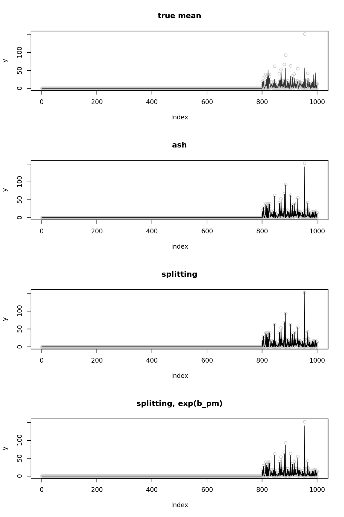
    if(i<=n_plot){
      par(mfrow=c(4,1))
      ylim = range(c(y,lambda,fit_split_ash_init$posterior$mean_exp_b,exp(fit_split_ash_init$posterior$mean_b)))
      plot(y,col='grey80',ylab='y',main='true mean',ylim=ylim)
      lines(lambda,col='grey20')
      plot(y,col='grey80',ylab='y',main='ash',ylim=ylim)
      lines(fit_ash$result$PosteriorMean)
      plot(y,col='grey80',ylab='y',main='splitting',ylim=ylim)
      lines(fit_split_ash_init$posterior$mean_exp_b)
      plot(y,col='grey80',ylab='y',main='splitting, exp(b_pm)',ylim=ylim)
      lines(exp(fit_split_ash_init$posterior$mean_b))
    }
    
  }
  return(list(mse_mean = mse_mean,mse_non0_mean = mse_non0_mean,sigma2=sigma2))
  
}

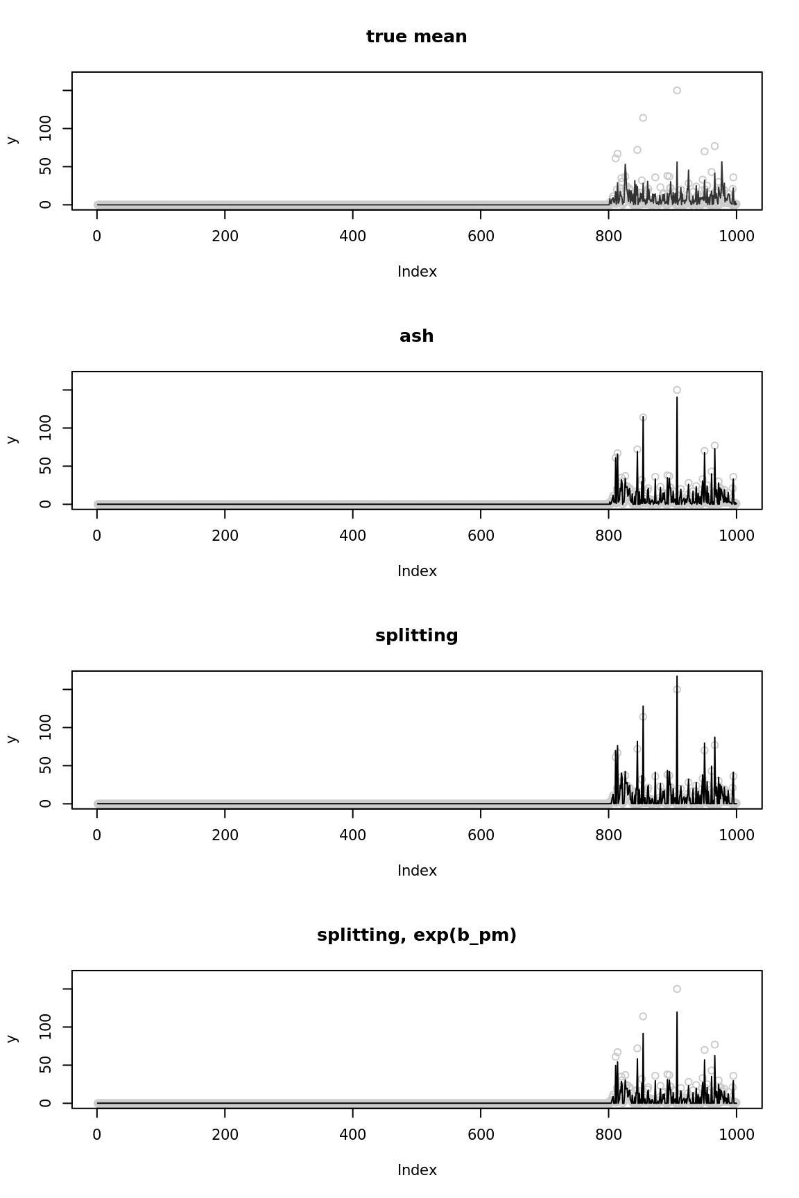
r = 10

res = simu_func(n_simu=10,n=1000,r = 10,n_plot = 10)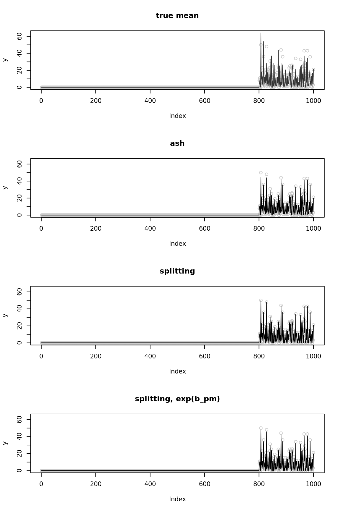

Past versions of unnamed-chunk-3-1.png

Version	Author	Date
7d3747e	DongyueXie	2022-11-29

Past versions of unnamed-chunk-3-2.png

Version	Author	Date
7d3747e	DongyueXie	2022-11-29

Past versions of unnamed-chunk-3-3.png

Version	Author	Date
7d3747e	DongyueXie	2022-11-29

Past versions of unnamed-chunk-3-4.png

Version	Author	Date
7d3747e	DongyueXie	2022-11-29

Past versions of unnamed-chunk-3-5.png

Version	Author	Date
7d3747e	DongyueXie	2022-11-29

Past versions of unnamed-chunk-3-6.png

Version	Author	Date
7d3747e	DongyueXie	2022-11-29

Past versions of unnamed-chunk-3-7.png

Version	Author	Date
7d3747e	DongyueXie	2022-11-29

Past versions of unnamed-chunk-3-8.png

Version	Author	Date
7d3747e	DongyueXie	2022-11-29

Past versions of unnamed-chunk-3-9.png

Version	Author	Date
7d3747e	DongyueXie	2022-11-29

Past versions of unnamed-chunk-3-10.png

Version	Author	Date
7d3747e	DongyueXie	2022-11-29

colMeans(res$mse_mean)

            ash           split split exp(b_pm) 
       5.519197        6.371801        5.822060 

colMeans(res$mse_non0_mean)

            ash           split split exp(b_pm) 
       27.59361        31.83897        29.09030 

r = 5

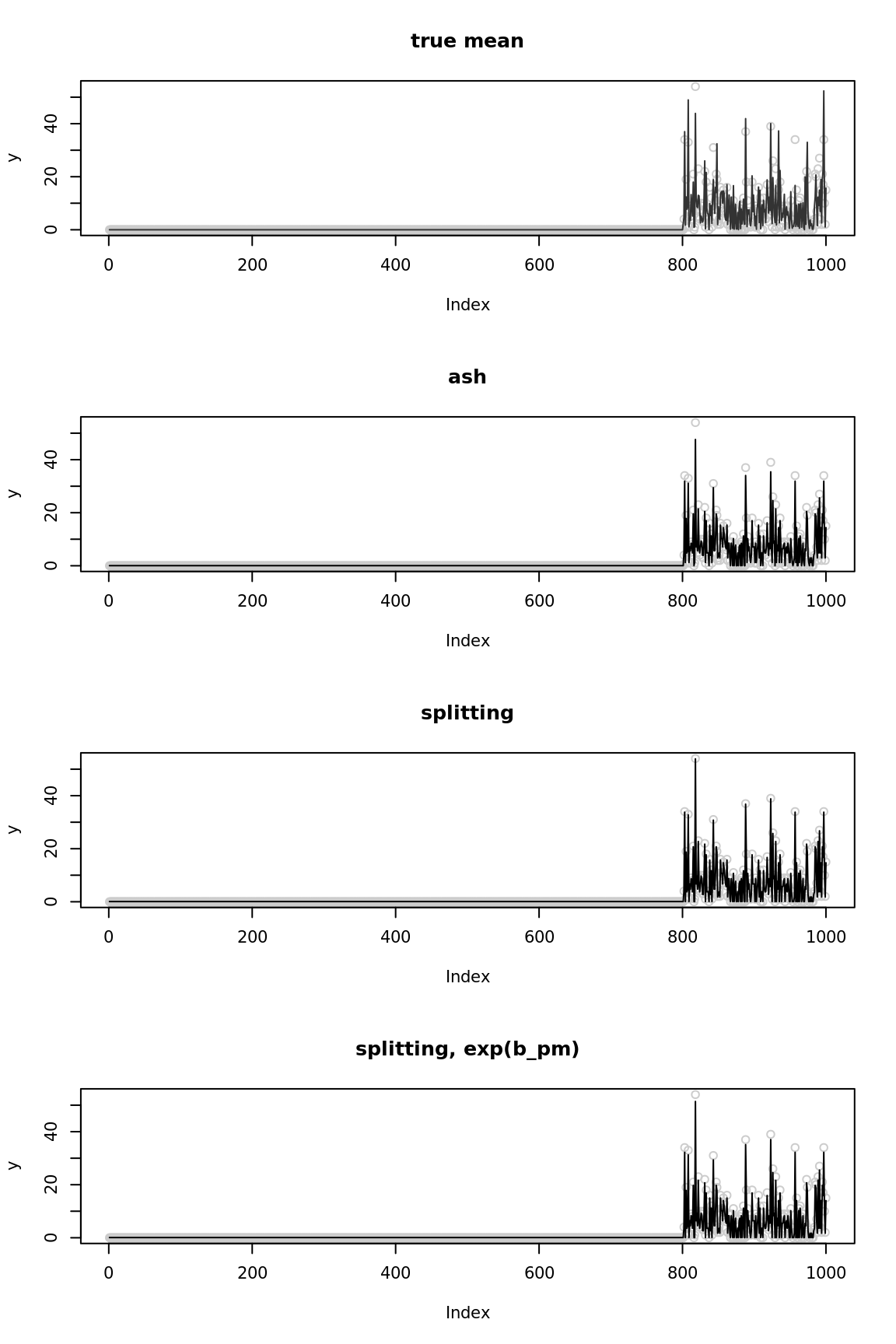
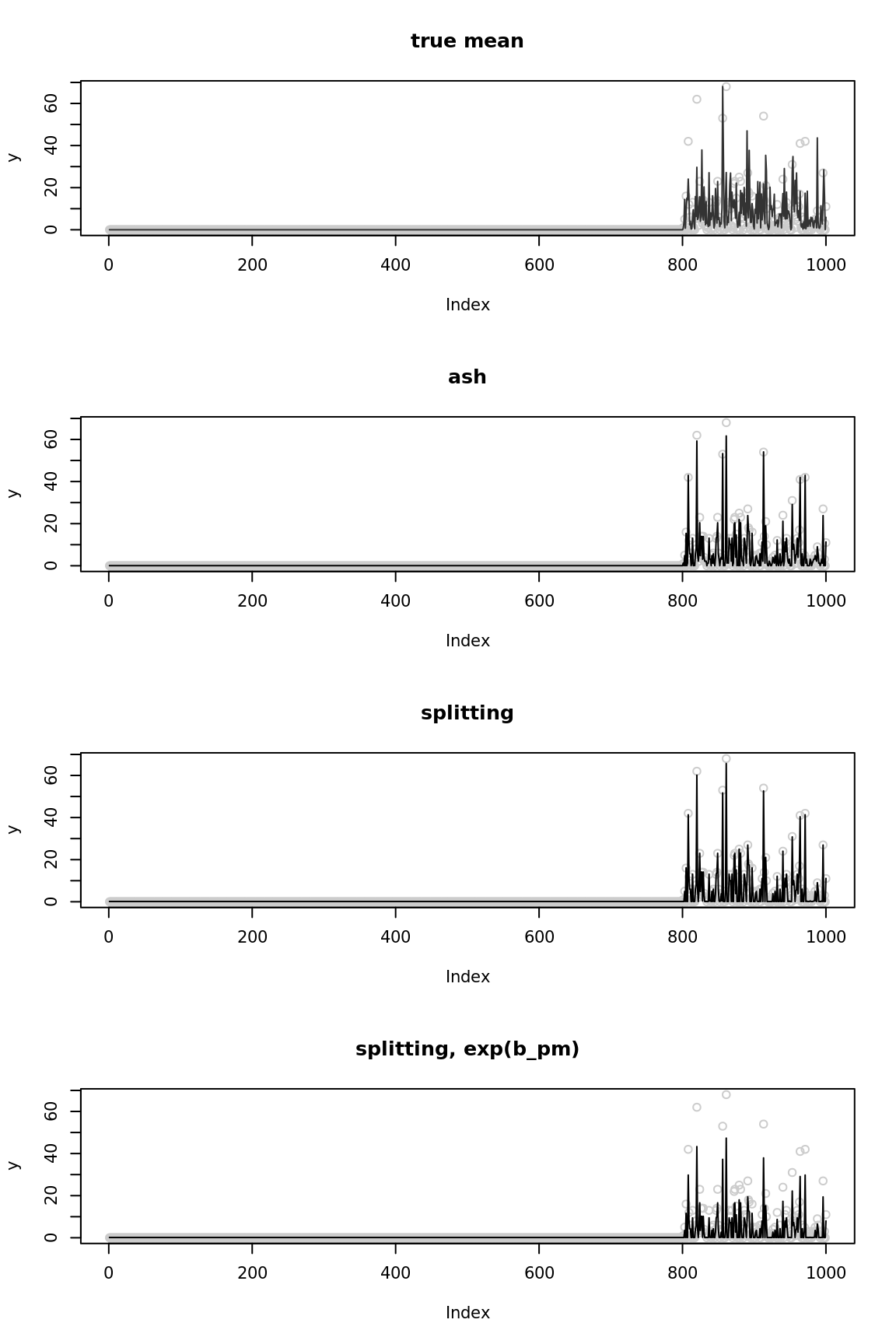
res = simu_func(n_simu=10,n=1000,r = 5,n_plot = 10)

Past versions of unnamed-chunk-4-1.png

Version	Author	Date
7d3747e	DongyueXie	2022-11-29
94d73ac	DongyueXie	2022-11-21

Past versions of unnamed-chunk-4-2.png

Version	Author	Date
7d3747e	DongyueXie	2022-11-29

Past versions of unnamed-chunk-4-3.png

Version	Author	Date
7d3747e	DongyueXie	2022-11-29

Past versions of unnamed-chunk-4-4.png

Version	Author	Date
7d3747e	DongyueXie	2022-11-29

Past versions of unnamed-chunk-4-5.png

Version	Author	Date
7d3747e	DongyueXie	2022-11-29

Past versions of unnamed-chunk-4-6.png

Version	Author	Date
7d3747e	DongyueXie	2022-11-29

Past versions of unnamed-chunk-4-7.png

Version	Author	Date
7d3747e	DongyueXie	2022-11-29

Past versions of unnamed-chunk-4-8.png

Version	Author	Date
7d3747e	DongyueXie	2022-11-29

Past versions of unnamed-chunk-4-9.png

Version	Author	Date
7d3747e	DongyueXie	2022-11-29

Past versions of unnamed-chunk-4-10.png

Version	Author	Date
7d3747e	DongyueXie	2022-11-29

colMeans(res$mse_mean)

            ash           split split exp(b_pm) 
       9.715968       11.669435        9.867543 

colMeans(res$mse_non0_mean)

            ash           split split exp(b_pm) 
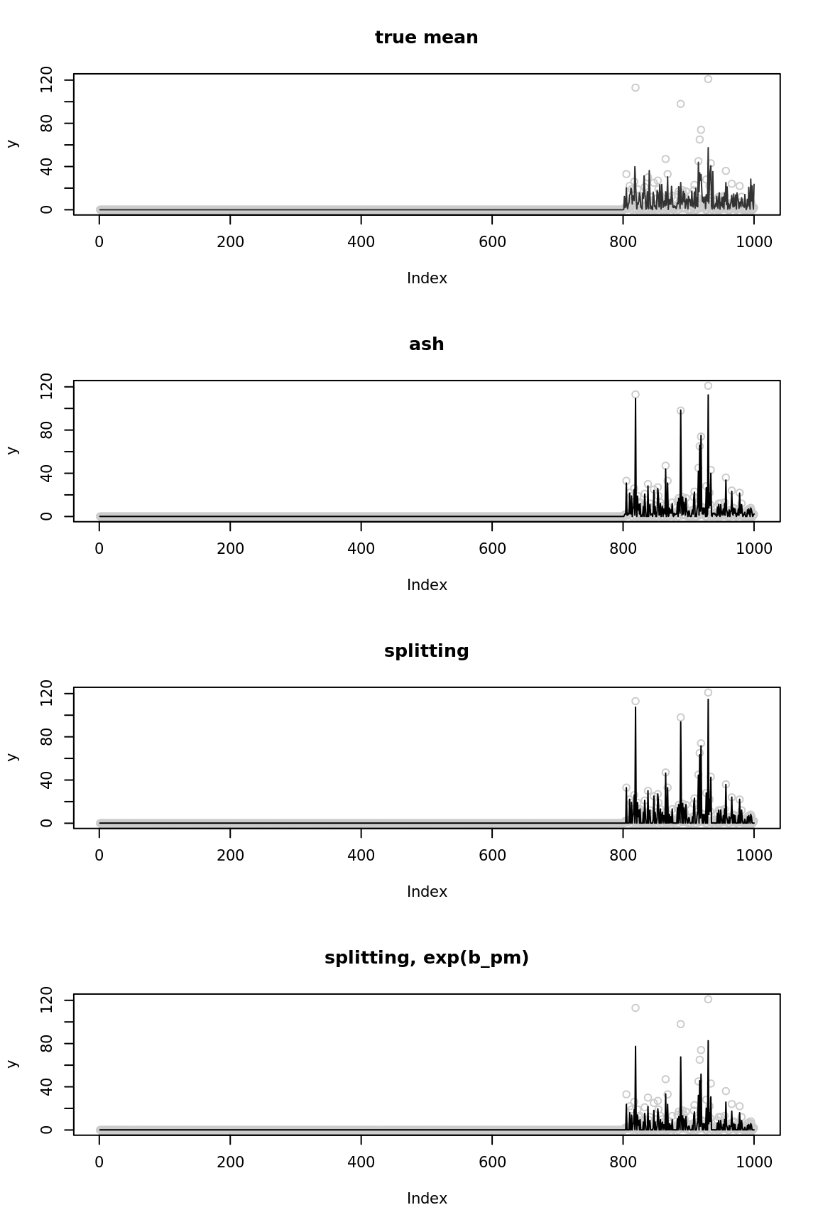
       48.57728        58.31219        49.30285 

r = 1

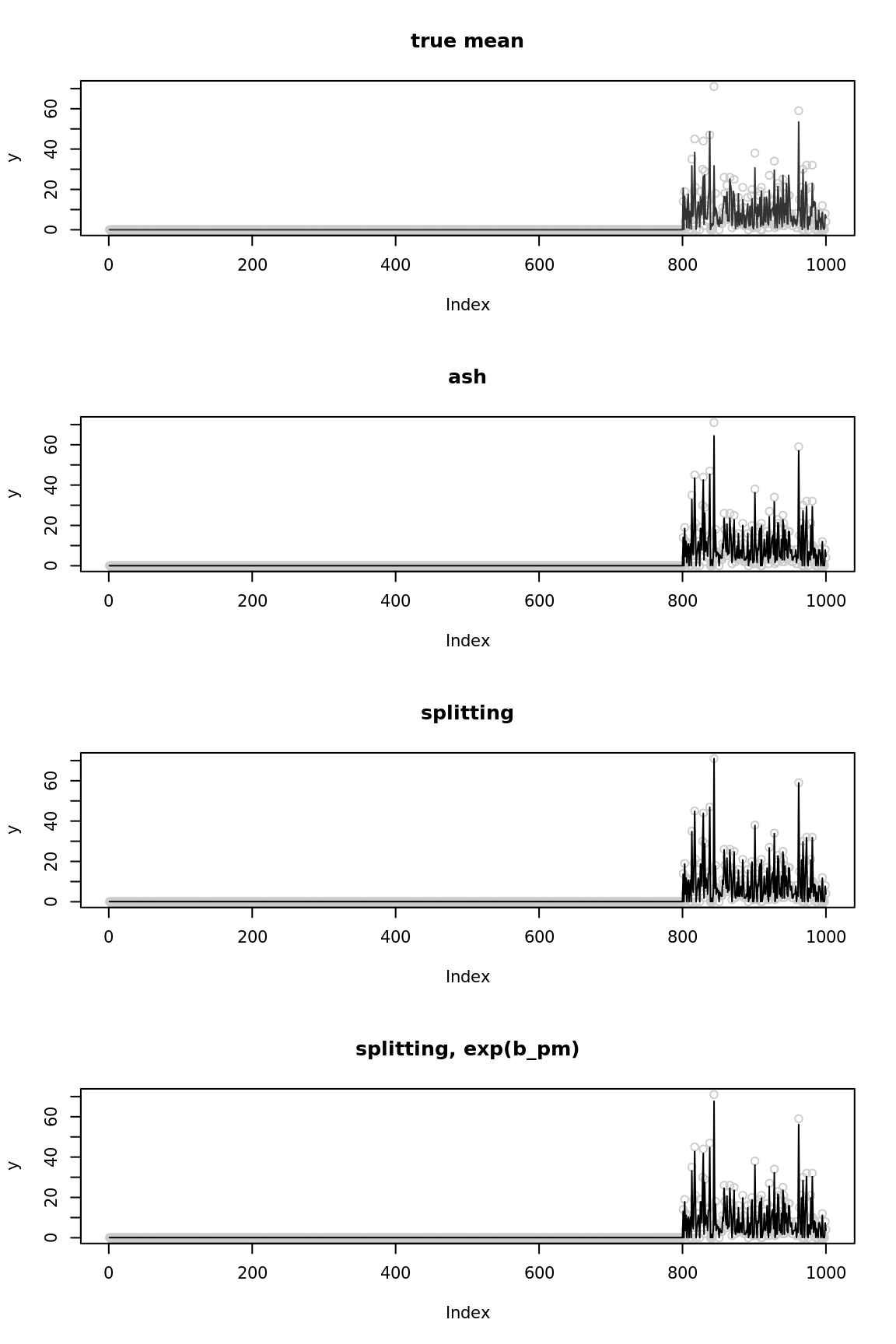
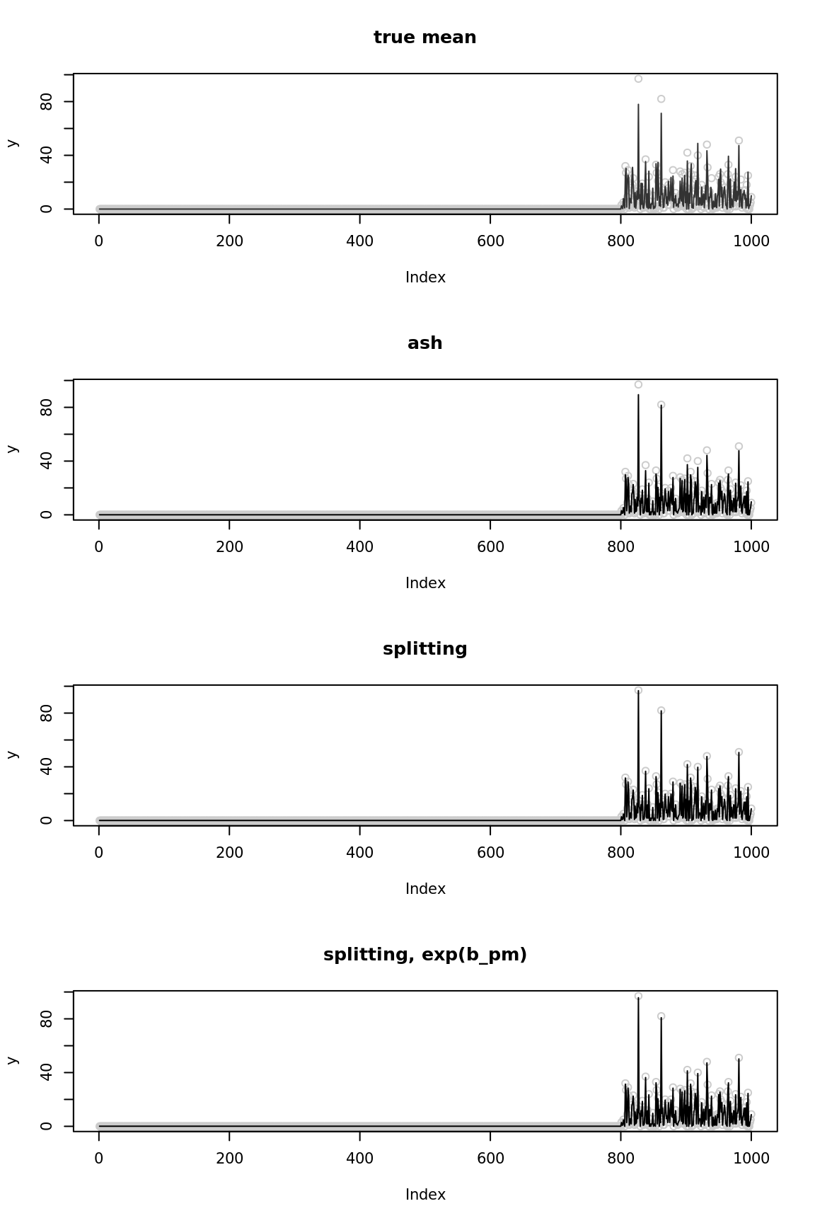
res = simu_func(n_simu=10,n=1000,r = 1,n_plot = 10)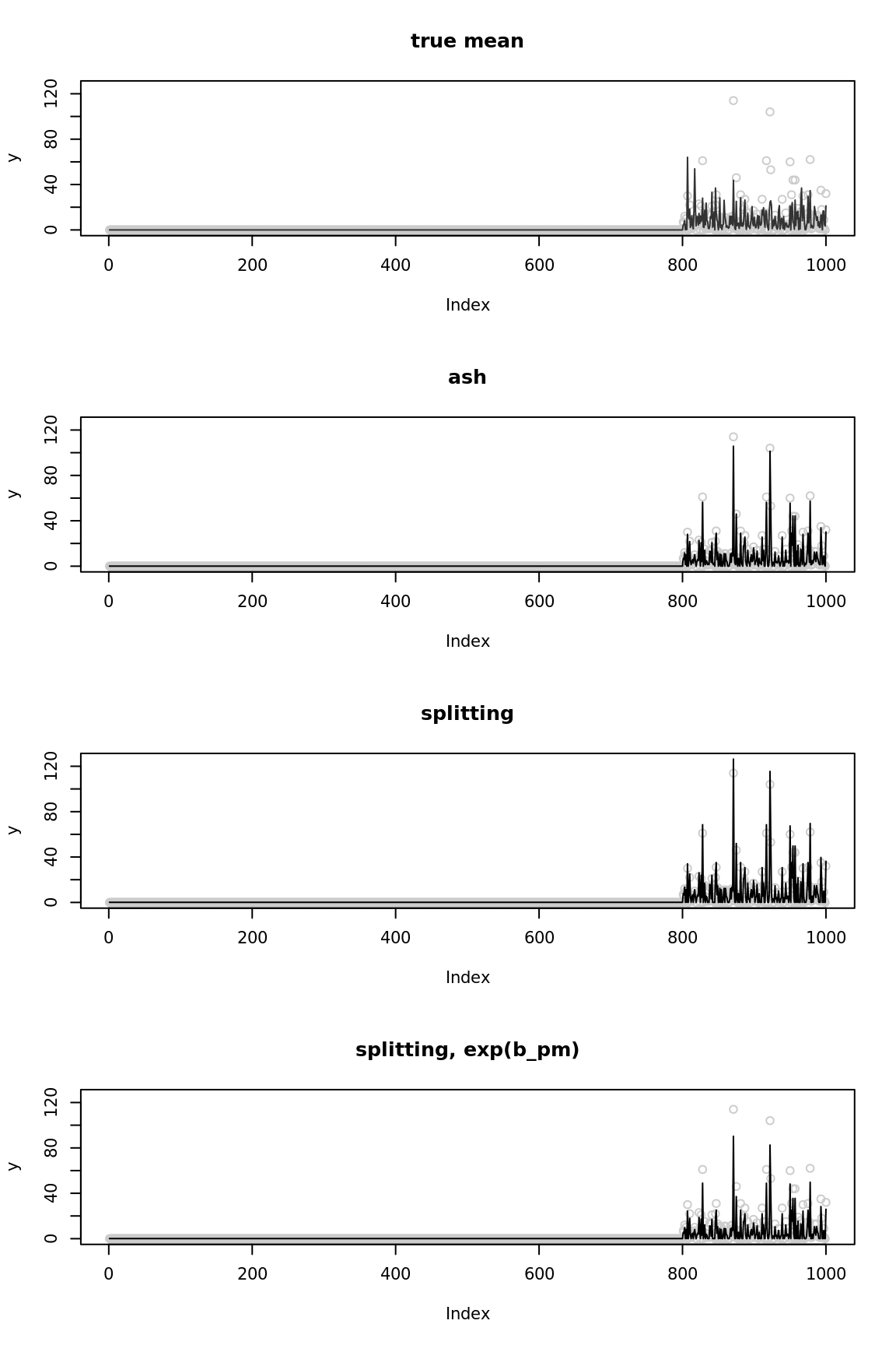

Past versions of unnamed-chunk-5-1.png

Version	Author	Date
7d3747e	DongyueXie	2022-11-29

Past versions of unnamed-chunk-5-2.png

Version	Author	Date
7d3747e	DongyueXie	2022-11-29

Past versions of unnamed-chunk-5-3.png

Version	Author	Date
7d3747e	DongyueXie	2022-11-29

Past versions of unnamed-chunk-5-4.png

Version	Author	Date
7d3747e	DongyueXie	2022-11-29

Past versions of unnamed-chunk-5-5.png

Version	Author	Date
7d3747e	DongyueXie	2022-11-29

Past versions of unnamed-chunk-5-6.png

Version	Author	Date
7d3747e	DongyueXie	2022-11-29

Past versions of unnamed-chunk-5-7.png

Version	Author	Date
7d3747e	DongyueXie	2022-11-29

Past versions of unnamed-chunk-5-8.png

Version	Author	Date
7d3747e	DongyueXie	2022-11-29

Past versions of unnamed-chunk-5-9.png

Version	Author	Date
7d3747e	DongyueXie	2022-11-29

Past versions of unnamed-chunk-5-10.png

Version	Author	Date
7d3747e	DongyueXie	2022-11-29

colMeans(res$mse_mean)

            ash           split split exp(b_pm) 
       30.42936        40.33983        24.16137 

colMeans(res$mse_non0_mean)

            ash           split split exp(b_pm) 
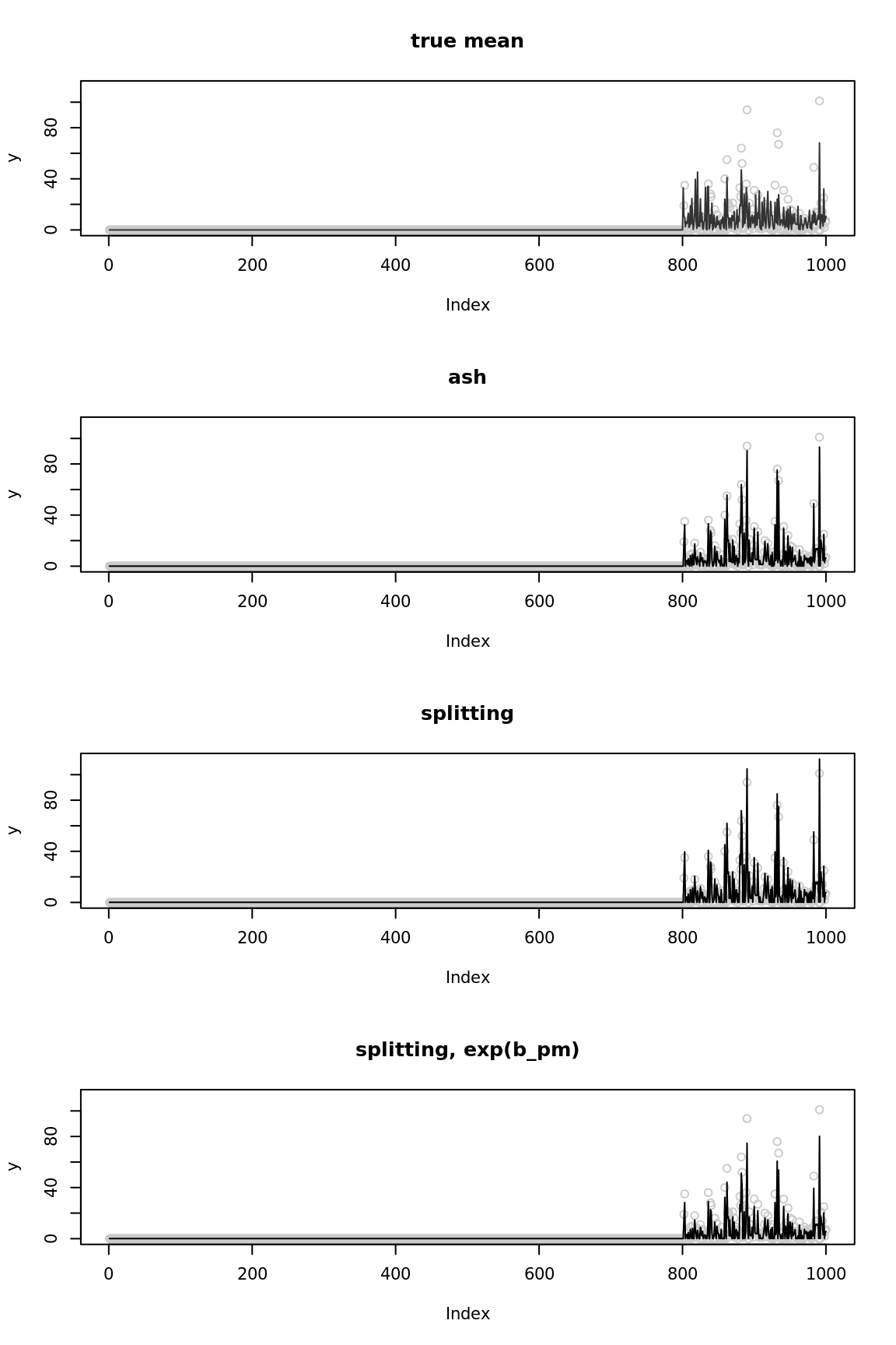
       152.1421        201.6679        120.7762 

r = 50

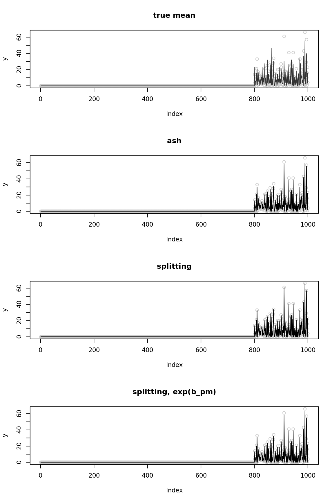
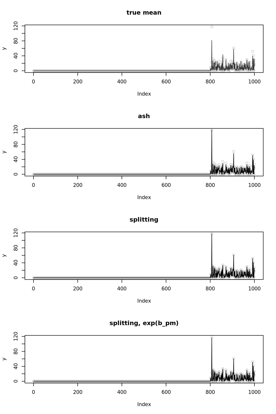
res = simu_func(n_simu=10,n=1000,r = 50,n_plot = 10)

Past versions of unnamed-chunk-6-1.png

Version	Author	Date
7d3747e	DongyueXie	2022-11-29
94d73ac	DongyueXie	2022-11-21

Past versions of unnamed-chunk-6-2.png

Version	Author	Date
7d3747e	DongyueXie	2022-11-29

Past versions of unnamed-chunk-6-3.png

Version	Author	Date
7d3747e	DongyueXie	2022-11-29

Past versions of unnamed-chunk-6-4.png

Version	Author	Date
7d3747e	DongyueXie	2022-11-29

Past versions of unnamed-chunk-6-5.png

Version	Author	Date
7d3747e	DongyueXie	2022-11-29

Past versions of unnamed-chunk-6-6.png

Version	Author	Date
7d3747e	DongyueXie	2022-11-29

Past versions of unnamed-chunk-6-7.png

Version	Author	Date
7d3747e	DongyueXie	2022-11-29

Past versions of unnamed-chunk-6-8.png

Version	Author	Date
7d3747e	DongyueXie	2022-11-29

Past versions of unnamed-chunk-6-9.png

Version	Author	Date
7d3747e	DongyueXie	2022-11-29

Past versions of unnamed-chunk-6-10.png

Version	Author	Date
7d3747e	DongyueXie	2022-11-29

colMeans(res$mse_mean)

            ash           split split exp(b_pm) 
       2.723380        2.905060        2.842274 

colMeans(res$mse_non0_mean)

            ash           split split exp(b_pm) 
       13.61450        14.50211        14.18819 

Session information

sessionInfo()

R version 4.2.1 (2022-06-23)
Platform: x86_64-pc-linux-gnu (64-bit)
Running under: Ubuntu 20.04.5 LTS

Matrix products: default
BLAS:   /usr/lib/x86_64-linux-gnu/blas/libblas.so.3.9.0
LAPACK: /usr/lib/x86_64-linux-gnu/lapack/liblapack.so.3.9.0

locale:
 [1] LC_CTYPE=C.UTF-8       LC_NUMERIC=C           LC_TIME=C.UTF-8       
 [4] LC_COLLATE=C.UTF-8     LC_MONETARY=C.UTF-8    LC_MESSAGES=C.UTF-8   
 [7] LC_PAPER=C.UTF-8       LC_NAME=C              LC_ADDRESS=C          
[10] LC_TELEPHONE=C         LC_MEASUREMENT=C.UTF-8 LC_IDENTIFICATION=C   

attached base packages:
[1] stats     graphics  grDevices utils     datasets  methods   base     

other attached packages:
[1] ashr_2.2-54     vebpm_0.3.1     workflowr_1.7.0

loaded via a namespace (and not attached):
 [1] Rcpp_1.0.9         horseshoe_0.2.0    invgamma_1.1       lattice_0.20-45   
 [5] nleqslv_3.3.3      getPass_0.2-2      ps_1.7.1           assertthat_0.2.1  
 [9] rprojroot_2.0.3    digest_0.6.29      utf8_1.2.2         truncnorm_1.0-8   
[13] R6_2.5.1           rootSolve_1.8.2.3  evaluate_0.17      highr_0.9         
[17] httr_1.4.4         ggplot2_3.3.6      pillar_1.8.1       rlang_1.0.6       
[21] rstudioapi_0.14    ebnm_1.0-9         irlba_2.3.5.1      nloptr_2.0.3      
[25] whisker_0.4        callr_3.7.2        jquerylib_0.1.4    Matrix_1.5-1      
[29] rmarkdown_2.17     splines_4.2.1      stringr_1.4.1      munsell_0.5.0     
[33] mixsqp_0.3-48      compiler_4.2.1     httpuv_1.6.6       xfun_0.33         
[37] pkgconfig_2.0.3    SQUAREM_2021.1     htmltools_0.5.3    tidyselect_1.2.0  
[41] tibble_3.1.8       matrixStats_0.62.0 fansi_1.0.3        dplyr_1.0.10      
[45] later_1.3.0        grid_4.2.1         jsonlite_1.8.2     gtable_0.3.1      
[49] lifecycle_1.0.3    DBI_1.1.3          git2r_0.30.1       magrittr_2.0.3    
[53] scales_1.2.1       ebpm_0.0.1.3       cli_3.4.1          stringi_1.7.8     
[57] cachem_1.0.6       fs_1.5.2           promises_1.2.0.1   bslib_0.4.0       
[61] generics_0.1.3     vctrs_0.4.2        trust_0.1-8        tools_4.2.1       
[65] glue_1.6.2         parallel_4.2.1     processx_3.7.0     fastmap_1.1.0     
[69] yaml_2.3.5         colorspace_2.0-3   deconvolveR_1.2-1  knitr_1.40        
[73] sass_0.4.2