pbmc3k 10X result
DongyueXie
2023-02-16
Last updated: 2023-02-16
Checks: 7 0
Knit directory: gsmash/
This reproducible R Markdown analysis was created with workflowr (version 1.7.0). The Checks tab describes the reproducibility checks that were applied when the results were created. The Past versions tab lists the development history.
Great! Since the R Markdown file has been committed to the Git repository, you know the exact version of the code that produced these results.
Great job! The global environment was empty. Objects defined in the global environment can affect the analysis in your R Markdown file in unknown ways. For reproduciblity it’s best to always run the code in an empty environment.
The command set.seed(20220606) was run prior to running
the code in the R Markdown file. Setting a seed ensures that any results
that rely on randomness, e.g. subsampling or permutations, are
reproducible.
Great job! Recording the operating system, R version, and package versions is critical for reproducibility.
Nice! There were no cached chunks for this analysis, so you can be confident that you successfully produced the results during this run.
Great job! Using relative paths to the files within your workflowr project makes it easier to run your code on other machines.
Great! You are using Git for version control. Tracking code development and connecting the code version to the results is critical for reproducibility.
The results in this page were generated with repository version 8545d58. See the Past versions tab to see a history of the changes made to the R Markdown and HTML files.
Note that you need to be careful to ensure that all relevant files for
the analysis have been committed to Git prior to generating the results
(you can use wflow_publish or
wflow_git_commit). workflowr only checks the R Markdown
file, but you know if there are other scripts or data files that it
depends on. Below is the status of the Git repository when the results
were generated:
Ignored files:
    Ignored:    .Rhistory
    Ignored:    .Rproj.user/

Untracked files:
    Untracked:  analysis/movielens.Rmd
    Untracked:  analysis/profiled_obj_for_b_splitting.Rmd
    Untracked:  code/poisson_STM/structure_plot.R
    Untracked:  data/ml-latest-small/
    Untracked:  data/pbmc3k_10x/
    Untracked:  output/droplet_iteration_results/
    Untracked:  output/ebpmf_pbmc3k_vga3_glmpca_init.rds
    Untracked:  output/pbmc3k_10x/
    Untracked:  output/pbmc3k_iteration_results/
    Untracked:  output/pbmc_no_constraint.rds
Note that any generated files, e.g. HTML, png, CSS, etc., are not included in this status report because it is ok for generated content to have uncommitted changes.
These are the previous versions of the repository in which changes were
made to the R Markdown (analysis/pbmc3k_10X_result.Rmd) and
HTML (docs/pbmc3k_10X_result.html) files. If you’ve
configured a remote Git repository (see ?wflow_git_remote),
click on the hyperlinks in the table below to view the files as they
were in that past version.
| File | Version | Author | Date | Message |
|---|---|---|---|---|
| Rmd | 8545d58 | DongyueXie | 2023-02-16 | wflow_publish("analysis/pbmc3k_10X_result.Rmd") |
Data
The pbmc3k data is from 10X, and I downloaded Gene/cell matrix(raw) dataset.
The quality control and cell types annotation are done by Seurat, following the tutorial here.
The resulting dataset has 2638 cells and 13714 genes.
pbmc3k = readRDS('data/pbmc3k_10x/pbmc3k.rds')
dim(pbmc3k$counts)
Loading required package: MatrixNULLThe cell types are
table(pbmc3k$cell_type)
 Naive CD4 T   CD14+ Mono Memory CD4 T            B        CD8 T FCGR3A+ Mono
         711          480          472          344          279          162
          NK           DC     Platelet
         144           32           14
Filter out genes
I filtered out genes that expressed in less than 10 cells, and no further preprocessing. The final data matrix is
library(stm)
library(Matrix)
counts = pbmc3k$counts
counts_filtered = counts[,colSums(counts!=0)>10]
dim(counts_filtered)
[1] 2638 10908pbmc3k_sparse = ebpmf_log(counts_filtered,flash_control = list())
saveRDS(pbmc3k_sparse,'pbmc3k_sparse.rds')
pbmc3k_nonnegL = ebpmf_log(counts_filtered,flash_control = list(ebnm.fn=c(ebnm::ebnm_point_exponential,ebnm::ebnm_point_normal),loadings_sign = 1))
saveRDS(pbmc3k_nonnegL,'pbmc3k_nonnegL_pe.rds')
pbmc3k_nonnegLF = ebpmf_log(counts_filtered,flash_control = list(ebnm.fn=c(ebnm::ebnm_point_exponential,ebnm::ebnm_point_exponential),factors_sign=1,loadings_sign = 1))
saveRDS(pbmc3k_nonnegLF,'pbmc3k_nonnegLF_pe.rds')
pbmc3k_nonnegL = ebpmf_log(counts_filtered,flash_control = list(ebnm.fn=c(ebnm::ebnm_unimodal_nonnegative,ebnm::ebnm_point_normal),loadings_sign = 1))
saveRDS(pbmc3k_nonnegL,'pbmc3k_nonnegL_un.rds')
pbmc3k_nonnegLF = ebpmf_log(counts_filtered,flash_control = list(ebnm.fn=c(ebnm::ebnm_unimodal_nonnegative,ebnm::ebnm_unimodal_nonnegative),factors_sign=1,loadings_sign = 1))
saveRDS(pbmc3k_nonnegLF,'pbmc3k_nonnegLF_un.rds')Model fitting
The model is the Empirical Bayes Poisson matrix factorization model,
and \(l_0\) is fixed at
log(rowMeans(Y)), \(f_0\)
is initialized at log(colSums(Y)/sum(l_0), then let the
model estiamtes \(f_0\) during
iterations.
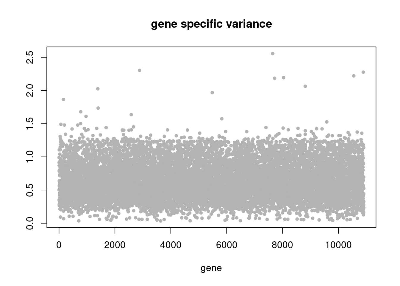
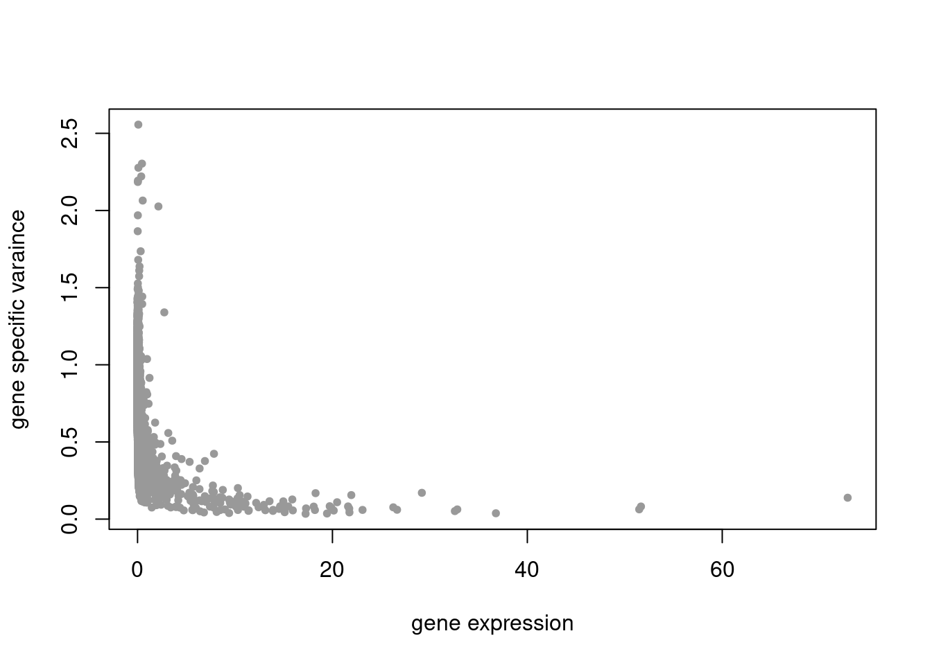
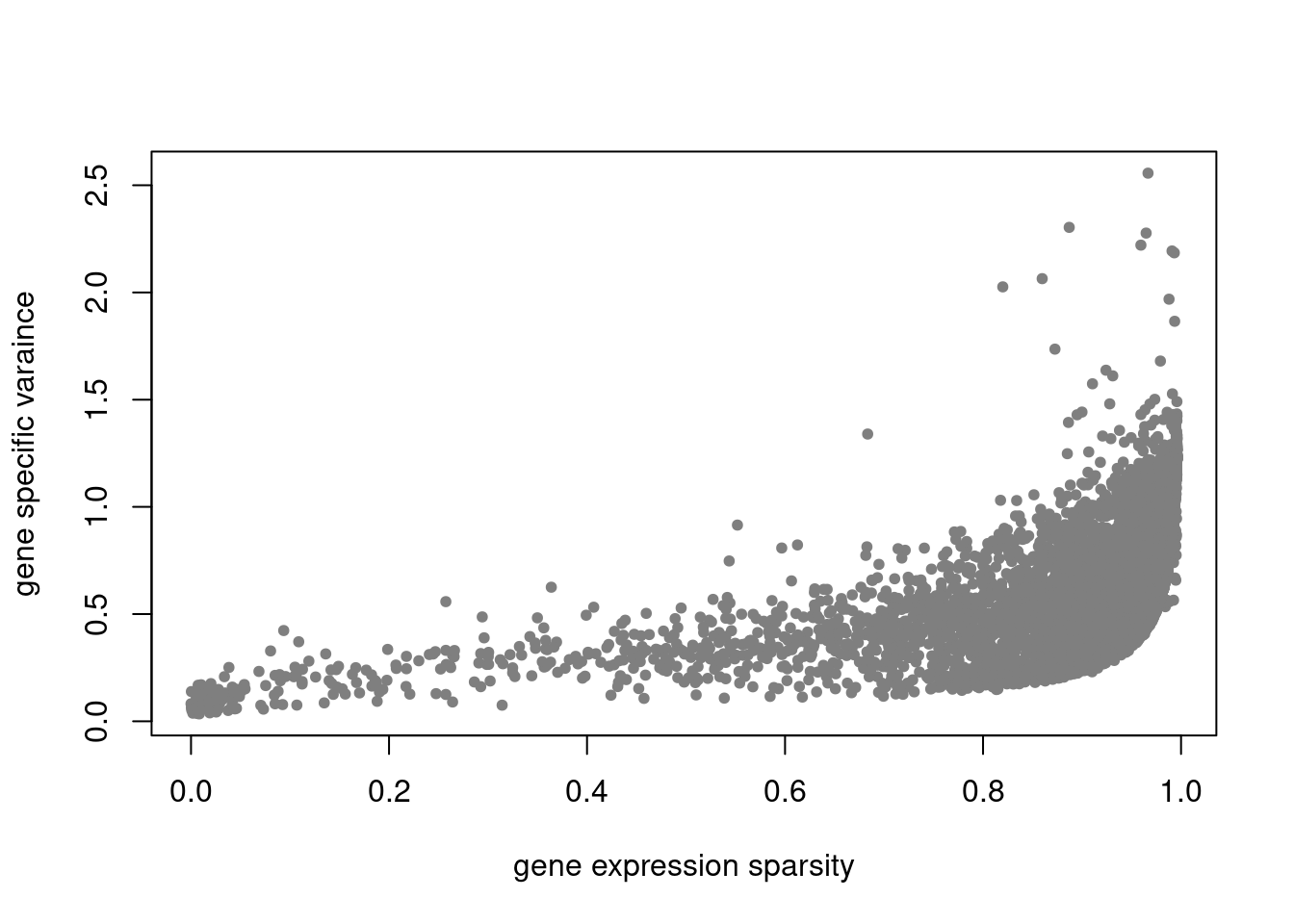
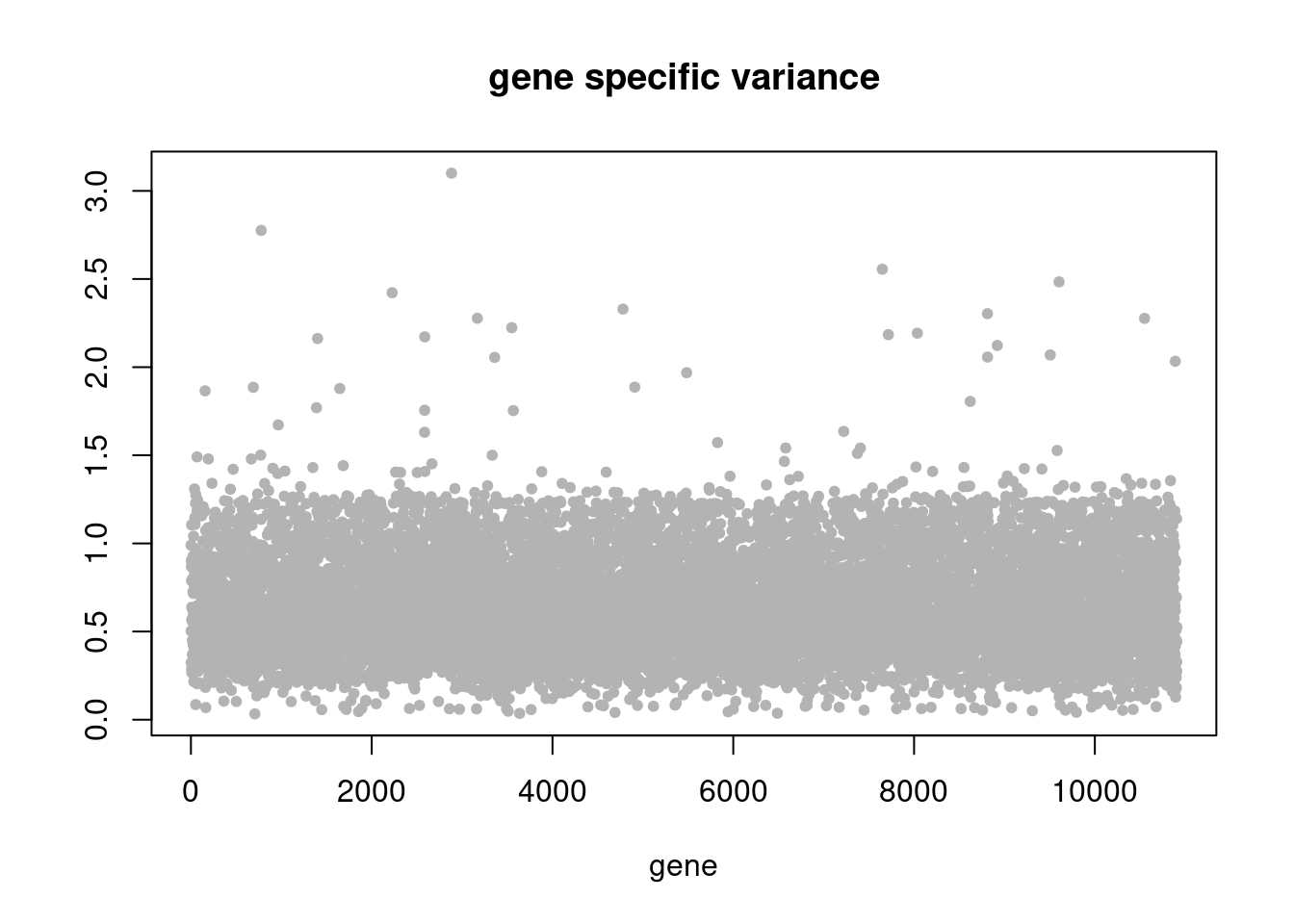
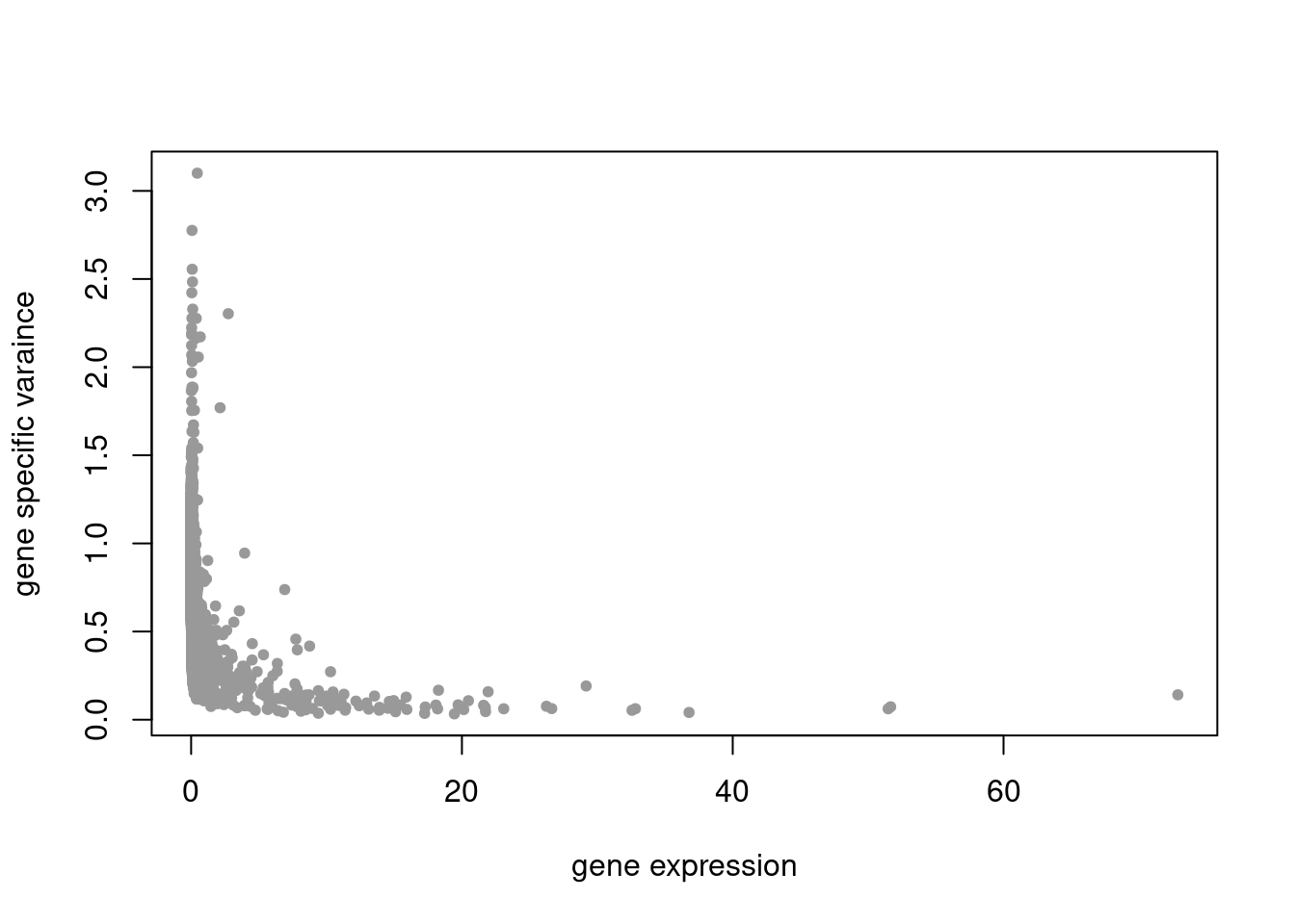
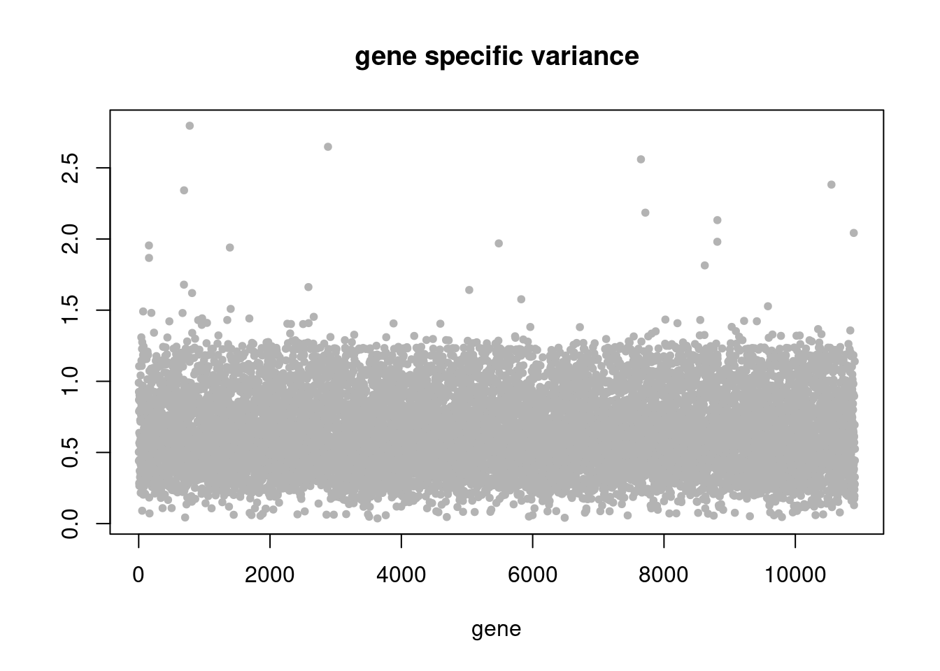
summary_plot = function(res){
plot(res$K_trace,ylab='',xlab='iterations',main='K over iterations',pch=20)
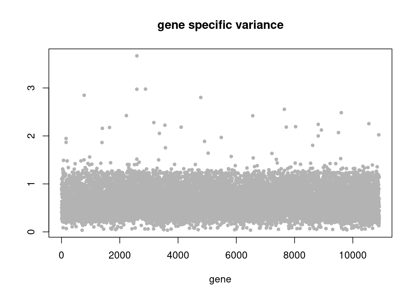
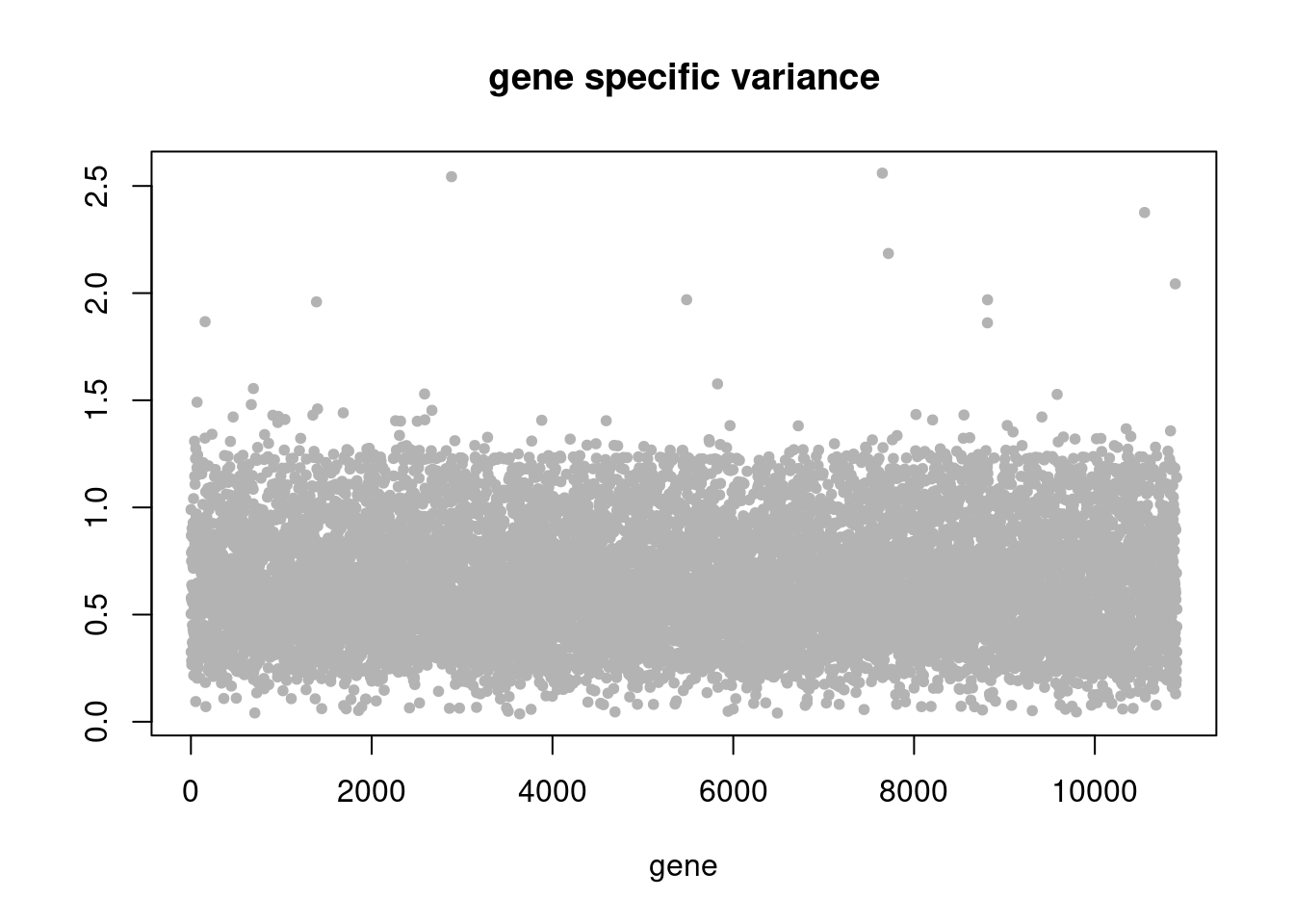
plot(res$sigma2,ylab='',xlab='gene',main = 'gene specific variance',pch=20,col='grey70')
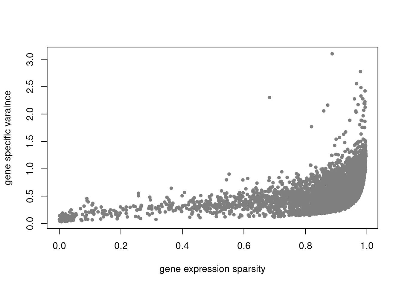
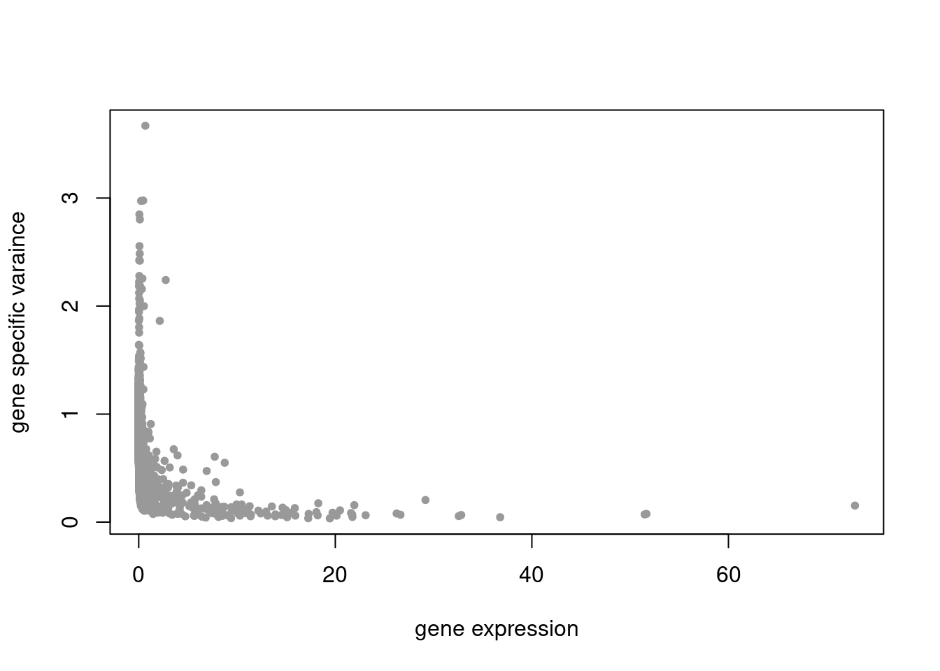
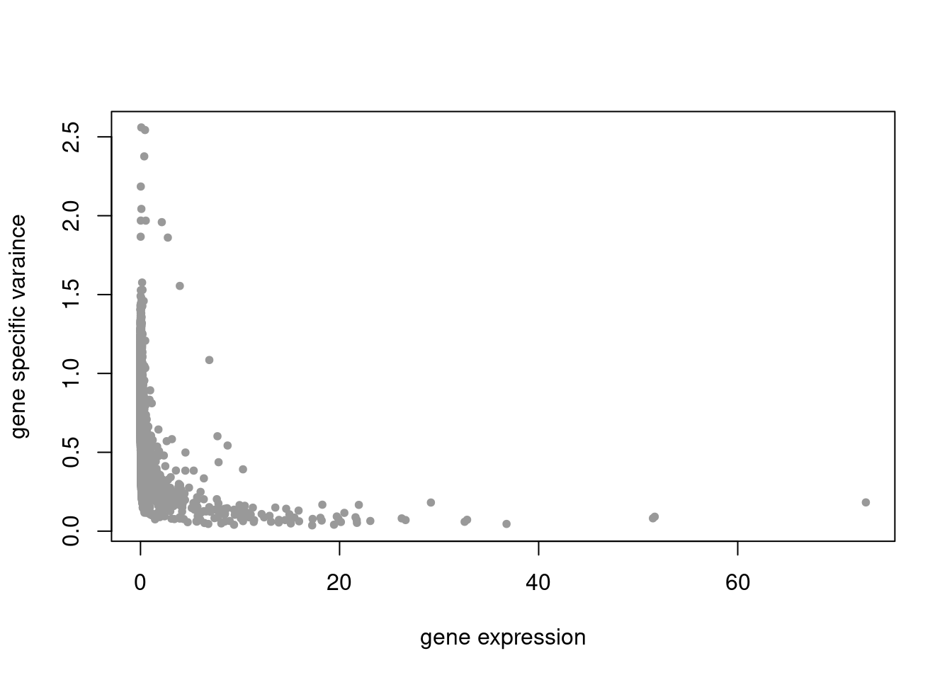
plot(colSums(counts_filtered/rowSums(counts_filtered)),res$sigma2,xlab='gene expression',ylab='gene specific varaince',pch=20,col='grey60')
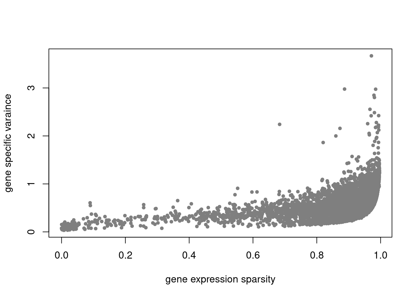
plot(colSums(counts_filtered==0)/nrow(counts_filtered),res$sigma2,xlab='gene expression sparsity',ylab='gene specific varaince',pch = 20, col='grey50')
}Sparse loadings and factors
source('code/poisson_STM/plot_factors.R')
pbmc3k_sparse = readRDS('output/pbmc3k_10x/pbmc3k_sparse.rds')
summary_plot(pbmc3k_sparse)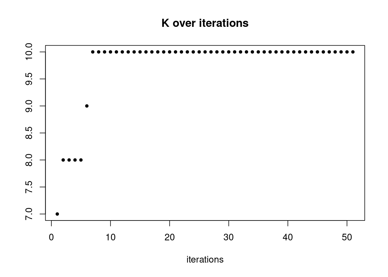
plot.factors(pbmc3k_sparse$fit_flash,pbmc3k$cell_type)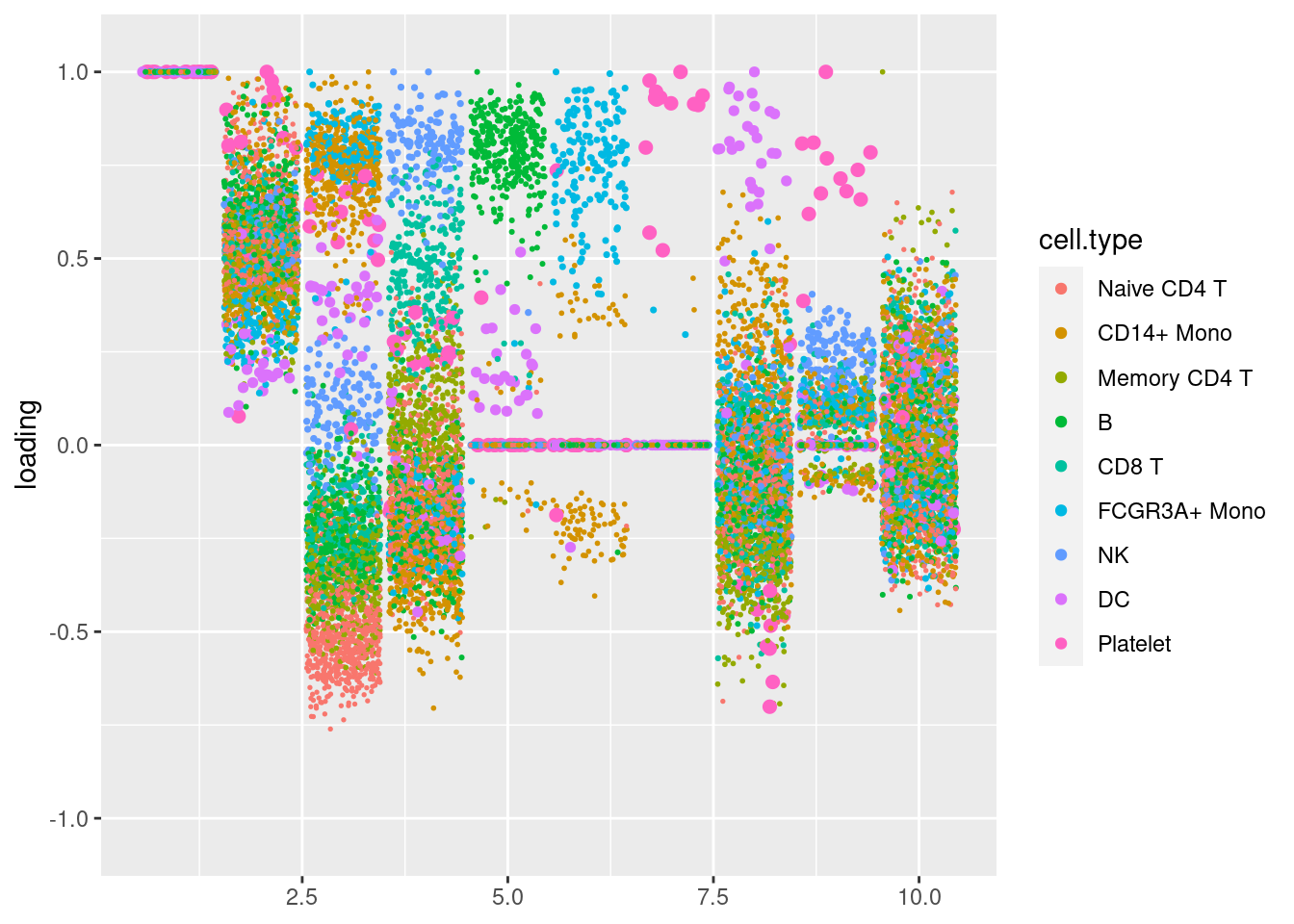
Nonnegative loadings with point exponential prior, and sparse factors
source('code/poisson_STM/structure_plot.R')
pbmc3k_nonnegL_pe = readRDS('output/pbmc3k_10x/pbmc3k_nonnegL_pe.rds')
summary_plot(pbmc3k_nonnegL_pe)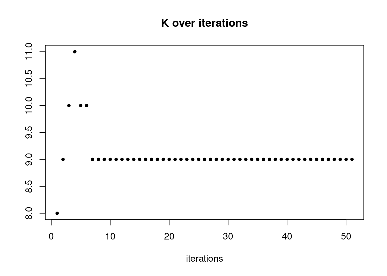
plot.factors(pbmc3k_nonnegL_pe$fit_flash,pbmc3k$cell_type,nonnegative = T)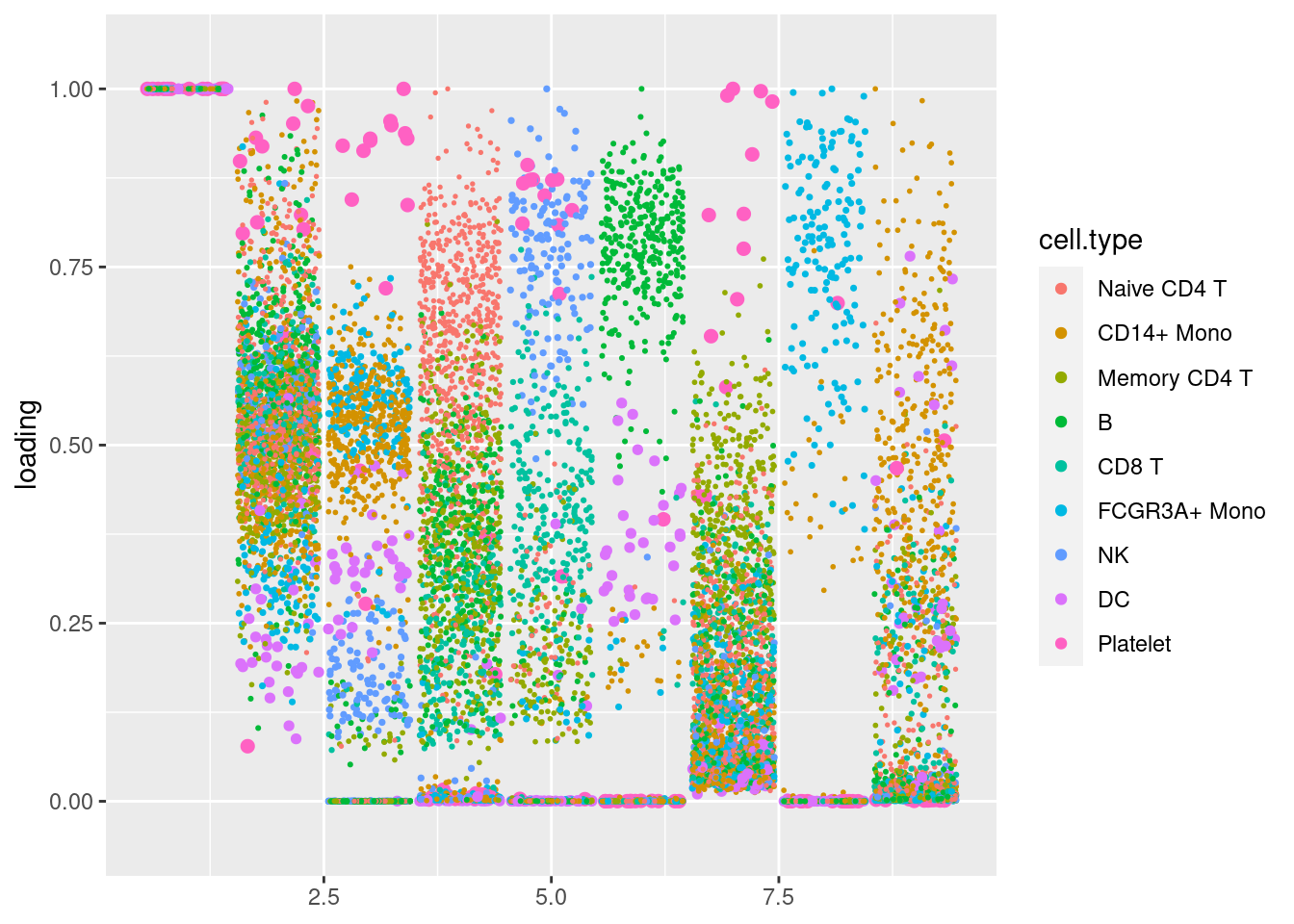
structure_plot_general(pbmc3k_nonnegL_pe$fit_flash$L.pm,pbmc3k_nonnegL_pe$fit_flash$F.pm,pbmc3k$cell_type,LD=T)Running tsne on 532 x 7 matrix.Running tsne on 363 x 7 matrix.Running tsne on 368 x 7 matrix.Running tsne on 259 x 7 matrix.Running tsne on 214 x 7 matrix.Running tsne on 119 x 7 matrix.Running tsne on 110 x 7 matrix.Running tsne on 24 x 7 matrix.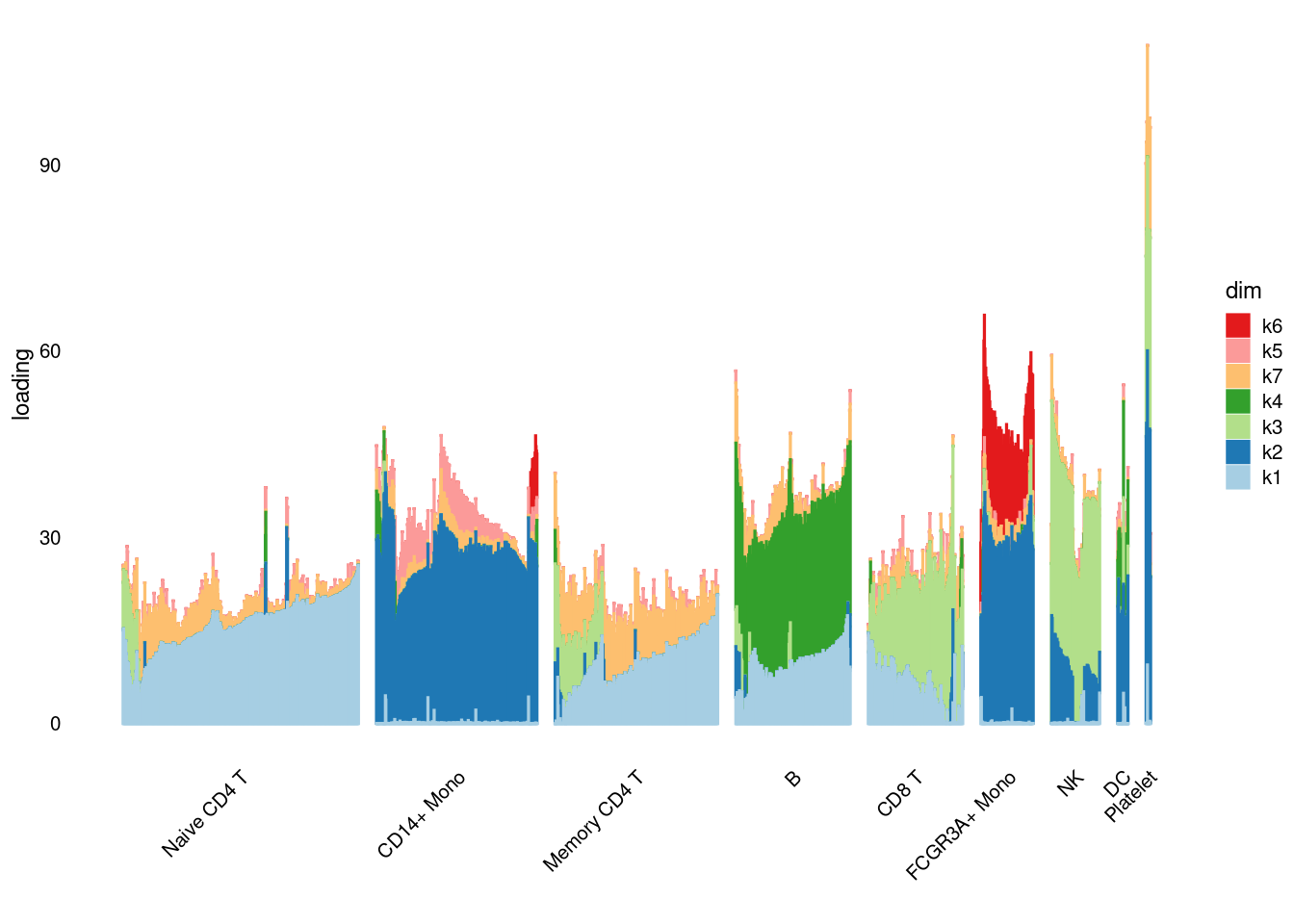
Nonnegative loadings with unimodal nonnegative prior, and sparse factors
pbmc3k_nonnegL_un = readRDS('output/pbmc3k_10x/pbmc3k_nonnegL_un.rds')summary_plot(pbmc3k_nonnegL_un)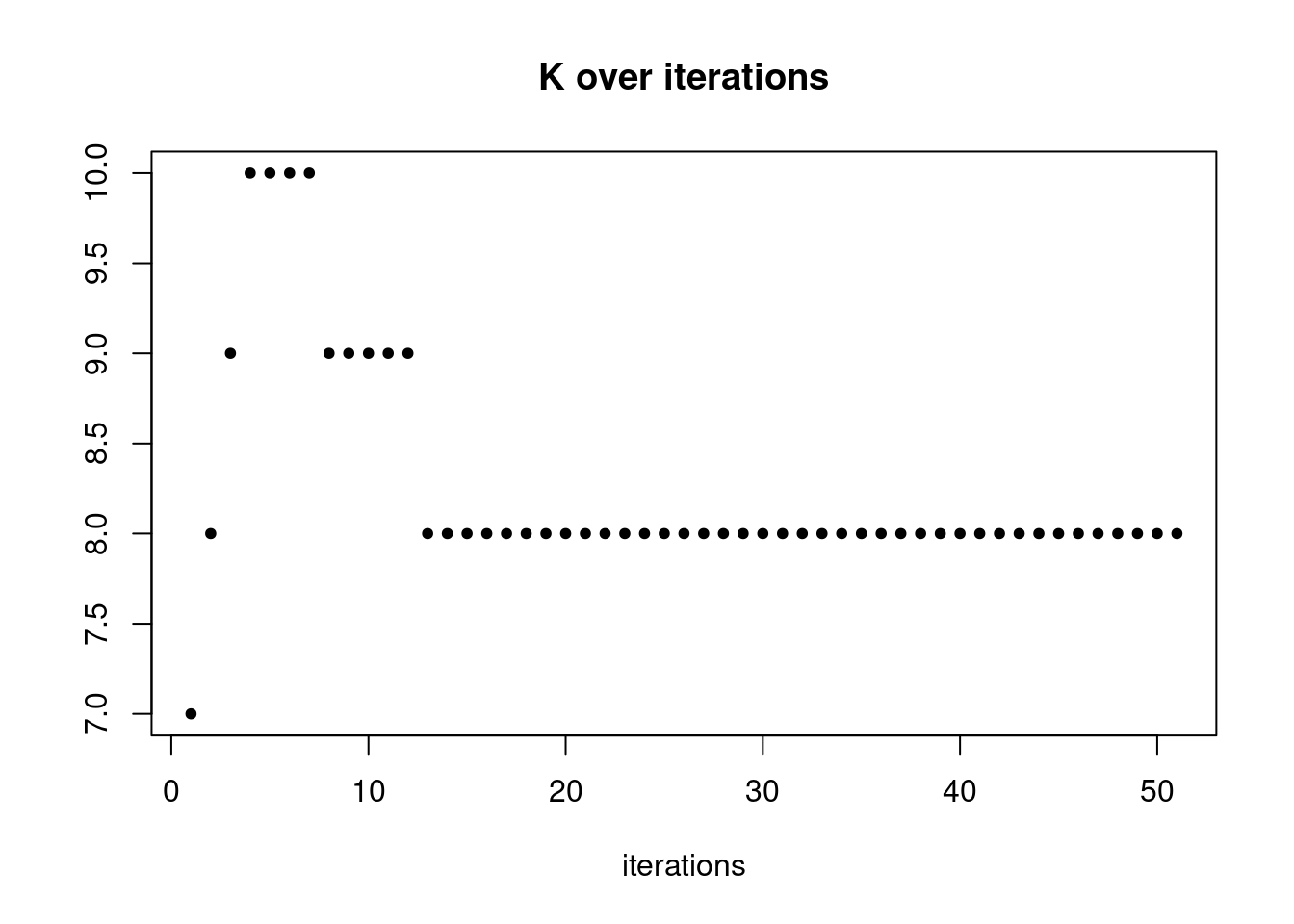
plot.factors(pbmc3k_nonnegL_un$fit_flash,pbmc3k$cell_type,nonnegative = T)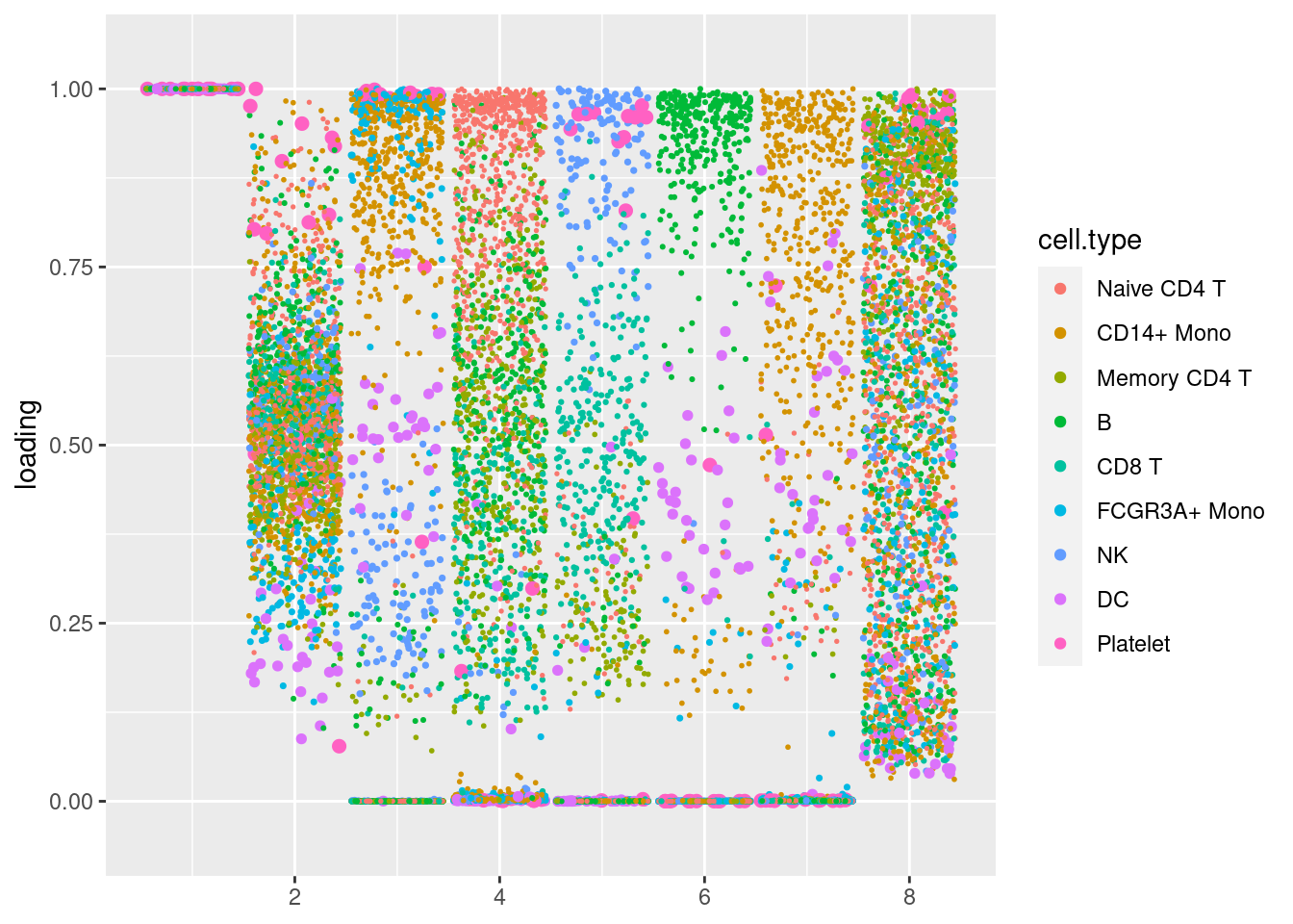
structure_plot_general(pbmc3k_nonnegL_un$fit_flash$L.pm,pbmc3k_nonnegL_un$fit_flash$F.pm,pbmc3k$cell_type,LD=T)Running tsne on 532 x 6 matrix.Running tsne on 363 x 6 matrix.Running tsne on 368 x 6 matrix.Running tsne on 259 x 6 matrix.Running tsne on 214 x 6 matrix.Running tsne on 119 x 6 matrix.Running tsne on 110 x 6 matrix.Running tsne on 24 x 6 matrix.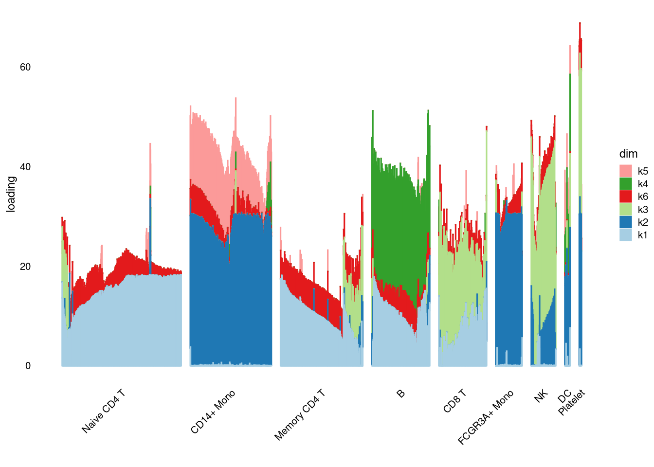
Nonnegative loadings and factors with point exponential prior
I got a warning message saying that
‘Warning message: In scale.EF(EF) : Fitting stopped after the initialization function failed to find a non-zero factor.’
pbmc3k_nonnegLF_pe = readRDS('output/pbmc3k_10x/pbmc3k_nonnegLF_pe.rds')summary_plot(pbmc3k_nonnegLF_pe)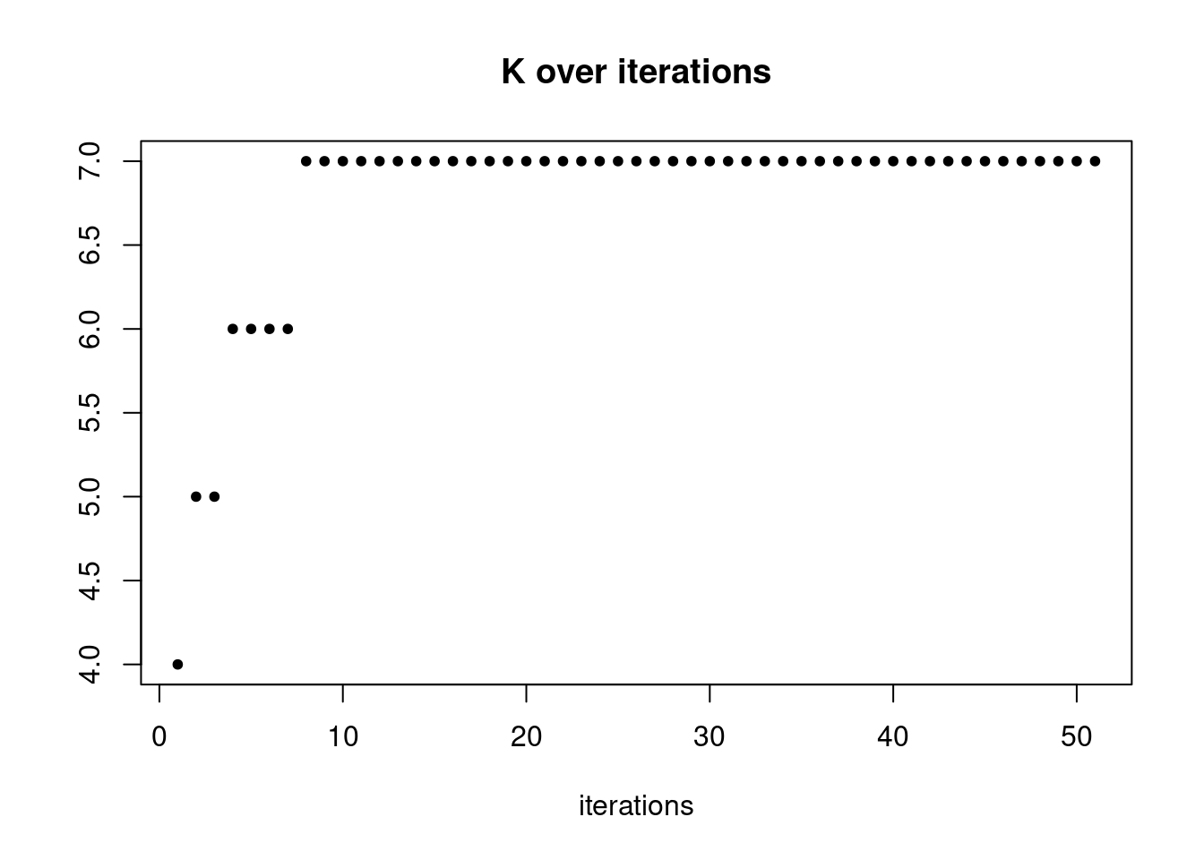


plot.factors(pbmc3k_nonnegLF_pe$fit_flash,pbmc3k$cell_type,nonnegative = T)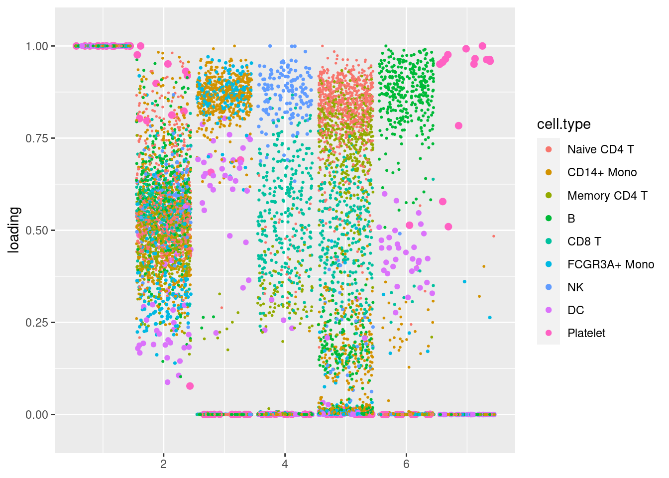
structure_plot_general(pbmc3k_nonnegLF_pe$fit_flash$L.pm,pbmc3k_nonnegLF_pe$fit_flash$F.pm,pbmc3k$cell_type,LD=T)Running tsne on 532 x 5 matrix.Running tsne on 363 x 5 matrix.Running tsne on 368 x 5 matrix.Running tsne on 259 x 5 matrix.Running tsne on 214 x 5 matrix.Running tsne on 119 x 5 matrix.Running tsne on 110 x 5 matrix.Running tsne on 24 x 5 matrix.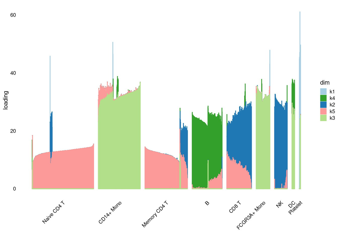
Nonnegative loadings and factors with unimodal nonnegative prior
I got a warning message saying that
‘Warning message: In scale.EF(EF) : Fitting stopped after the initialization function failed to find a non-zero factor.’
pbmc3k_nonnegLF_un = readRDS('output/pbmc3k_10x/pbmc3k_nonnegLF_un.rds')summary_plot(pbmc3k_nonnegLF_un)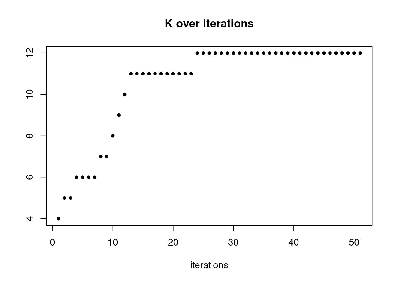

plot.factors(pbmc3k_nonnegLF_un$fit_flash,pbmc3k$cell_type,nonnegative = T)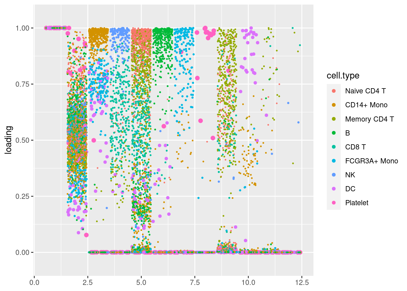
structure_plot_general(pbmc3k_nonnegLF_un$fit_flash$L.pm,pbmc3k_nonnegLF_un$fit_flash$F.pm,pbmc3k$cell_type,LD=T)Running tsne on 532 x 10 matrix.Running tsne on 363 x 10 matrix.Running tsne on 368 x 10 matrix.Running tsne on 259 x 10 matrix.Running tsne on 214 x 10 matrix.Running tsne on 119 x 10 matrix.Running tsne on 110 x 10 matrix.Running tsne on 24 x 10 matrix.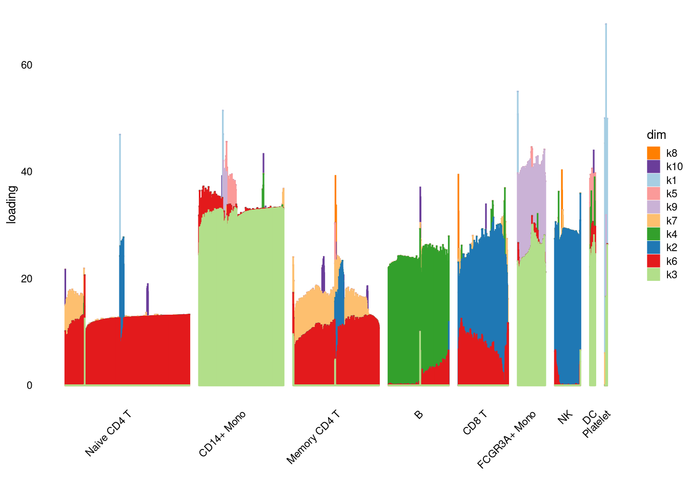
sessionInfo()R version 4.2.2 Patched (2022-11-10 r83330)
Platform: x86_64-pc-linux-gnu (64-bit)
Running under: Ubuntu 22.04.1 LTS
Matrix products: default
BLAS: /usr/lib/x86_64-linux-gnu/openblas-pthread/libblas.so.3
LAPACK: /usr/lib/x86_64-linux-gnu/openblas-pthread/libopenblasp-r0.3.20.so
locale:
[1] LC_CTYPE=en_US.UTF-8 LC_NUMERIC=C
[3] LC_TIME=en_US.UTF-8 LC_COLLATE=en_US.UTF-8
[5] LC_MONETARY=en_US.UTF-8 LC_MESSAGES=en_US.UTF-8
[7] LC_PAPER=en_US.UTF-8 LC_NAME=C
[9] LC_ADDRESS=C LC_TELEPHONE=C
[11] LC_MEASUREMENT=en_US.UTF-8 LC_IDENTIFICATION=C
attached base packages:
[1] stats graphics grDevices utils datasets methods base
other attached packages:
[1] fastTopics_0.6-142 ggplot2_3.4.0 stm_2.0.2 Matrix_1.5-3
[5] workflowr_1.7.0
loaded via a namespace (and not attached):
[1] Rtsne_0.16 ebpm_0.0.1.3 colorspace_2.0-3
[4] smashr_1.3-6 ellipsis_0.3.2 mr.ash_0.1-87
[7] rprojroot_2.0.3 fs_1.5.2 rstudioapi_0.14
[10] farver_2.1.1 MatrixModels_0.5-1 ggrepel_0.9.2
[13] fansi_1.0.3 codetools_0.2-19 splines_4.2.2
[16] cachem_1.0.6 knitr_1.41 jsonlite_1.8.4
[19] nloptr_2.0.3 mcmc_0.9-7 ashr_2.2-54
[22] smashrgen_1.1.5 uwot_0.1.14 compiler_4.2.2
[25] httr_1.4.4 RcppZiggurat_0.1.6 fastmap_1.1.0
[28] lazyeval_0.2.2 cli_3.4.1 later_1.3.0
[31] htmltools_0.5.4 quantreg_5.94 prettyunits_1.1.1
[34] tools_4.2.2 coda_0.19-4 gtable_0.3.1
[37] glue_1.6.2 reshape2_1.4.4 dplyr_1.0.10
[40] Rcpp_1.0.9 softImpute_1.4-1 jquerylib_0.1.4
[43] vctrs_0.5.1 iterators_1.0.14 wavethresh_4.7.2
[46] xfun_0.35 stringr_1.5.0 ps_1.7.2
[49] trust_0.1-8 lifecycle_1.0.3 irlba_2.3.5.1
[52] NNLM_0.4.4 getPass_0.2-2 MASS_7.3-58.2
[55] scales_1.2.1 hms_1.1.2 promises_1.2.0.1
[58] parallel_4.2.2 SparseM_1.81 yaml_2.3.6
[61] pbapply_1.6-0 sass_0.4.4 stringi_1.7.8
[64] SQUAREM_2021.1 highr_0.9 deconvolveR_1.2-1
[67] foreach_1.5.2 caTools_1.18.2 truncnorm_1.0-8
[70] shape_1.4.6 horseshoe_0.2.0 rlang_1.0.6
[73] pkgconfig_2.0.3 matrixStats_0.63.0 bitops_1.0-7
[76] ebnm_1.0-12 evaluate_0.19 lattice_0.20-45
[79] invgamma_1.1 purrr_0.3.5 labeling_0.4.2
[82] htmlwidgets_1.6.0 Rfast_2.0.6 cowplot_1.1.1
[85] processx_3.8.0 tidyselect_1.2.0 plyr_1.8.8
[88] magrittr_2.0.3 R6_2.5.1 generics_0.1.3
[91] pillar_1.8.1 whisker_0.4.1 withr_2.5.0
[94] survival_3.5-0 mixsqp_0.3-48 tibble_3.1.8
[97] crayon_1.5.2 utf8_1.2.2 plotly_4.10.1
[100] rmarkdown_2.19 progress_1.2.2 grid_4.2.2
[103] data.table_1.14.6 callr_3.7.3 git2r_0.30.1
[106] digest_0.6.31 vebpm_0.4.1 tidyr_1.2.1
[109] httpuv_1.6.7 MCMCpack_1.6-3 RcppParallel_5.1.5
[112] munsell_0.5.0 glmnet_4.1-6 viridisLite_0.4.1
[115] flashier_0.2.34 bslib_0.4.2 quadprog_1.5-8