poisson smooth split local optimum
DongyueXie
2023-02-07
Last updated: 2023-02-07
Checks: 7 0
Knit directory: gsmash/
This reproducible R Markdown analysis was created with workflowr (version 1.7.0). The Checks tab describes the reproducibility checks that were applied when the results were created. The Past versions tab lists the development history.
Great! Since the R Markdown file has been committed to the Git repository, you know the exact version of the code that produced these results.
Great job! The global environment was empty. Objects defined in the global environment can affect the analysis in your R Markdown file in unknown ways. For reproduciblity it’s best to always run the code in an empty environment.
The command set.seed(20220606) was run prior to running
the code in the R Markdown file. Setting a seed ensures that any results
that rely on randomness, e.g. subsampling or permutations, are
reproducible.
Great job! Recording the operating system, R version, and package versions is critical for reproducibility.
Nice! There were no cached chunks for this analysis, so you can be confident that you successfully produced the results during this run.
Great job! Using relative paths to the files within your workflowr project makes it easier to run your code on other machines.
Great! You are using Git for version control. Tracking code development and connecting the code version to the results is critical for reproducibility.
The results in this page were generated with repository version a77fd7f. See the Past versions tab to see a history of the changes made to the R Markdown and HTML files.
Note that you need to be careful to ensure that all relevant files for
the analysis have been committed to Git prior to generating the results
(you can use wflow_publish or
wflow_git_commit). workflowr only checks the R Markdown
file, but you know if there are other scripts or data files that it
depends on. Below is the status of the Git repository when the results
were generated:
Ignored files:
    Ignored:    .Rhistory
    Ignored:    .Rproj.user/

Untracked files:
    Untracked:  analysis/movielens.Rmd
    Untracked:  analysis/profiled_obj_for_b_splitting.Rmd
    Untracked:  code/binomial_mean/binomial_smooth_splitting.R
    Untracked:  code/binomial_mean/test_binomial.R
    Untracked:  code/poisson_smooth/pois_reg_splitting.R
    Untracked:  data/ml-latest-small/
    Untracked:  output/droplet_iteration_results/
    Untracked:  output/ebpmf_pbmc3k_vga3_glmpca_init.rds
    Untracked:  output/pbmc3k_iteration_results/
    Untracked:  output/pbmc_no_constraint.rds

Unstaged changes:
    Modified:   analysis/index.Rmd
    Modified:   code/binomial_mean/binomial_mean_splitting.R
Note that any generated files, e.g. HTML, png, CSS, etc., are not included in this status report because it is ok for generated content to have uncommitted changes.
These are the previous versions of the repository in which changes were
made to the R Markdown
(analysis/poisson_smooth_split_local_optimum.Rmd) and HTML
(docs/poisson_smooth_split_local_optimum.html) files. If
you’ve configured a remote Git repository (see
?wflow_git_remote), click on the hyperlinks in the table
below to view the files as they were in that past version.
| File | Version | Author | Date | Message |
|---|---|---|---|---|
| Rmd | a77fd7f | DongyueXie | 2023-02-07 | wflow_publish("analysis/poisson_smooth_split_local_optimum.Rmd") |
Introduction
\[y_i\sim Poisson(exp(\mu_j)),\mu_j|b_j\sim N(b_j,\sigma^2),b\sim g(\cdot).\]
where \(g(\cdot)\) is a wavelet prior.
A simple block function
library(smashrgen)Loading required package: smashrLoading required package: ashrLoading required package: caToolsLoading required package: MASSLoading required package: wavethreshWaveThresh: R wavelet software, release 4.7.2, installedCopyright Guy Nason and others 1993-2022Note: nlevels has been renamed to nlevelsWTlibrary(wavethresh)
set.seed(12345)
n=2^9
sigma=0
mu=c(rep(0.3,n/4), rep(3, n/4), rep(10, n/4), rep(0.3, n/4))
x = rpois(n,exp(log(mu)+rnorm(n,sd=sigma)))
fit = pois_smooth_split(x,maxiter=300,verbose = T,tol=1e-10)[1] "Done iter 10 obj = -1056.96579525788"
[1] "Done iter 20 obj = -1044.11354637971"
[1] "Done iter 30 obj = -1040.86127751977"
[1] "Done iter 40 obj = -1039.53387402167"
[1] "Done iter 50 obj = -1038.85469459227"
[1] "Done iter 60 obj = -1038.45884469515"
[1] "Done iter 70 obj = -1038.20785536043"
[1] "Done iter 80 obj = -1038.03908581062"
[1] "Done iter 90 obj = -1037.92058752612"
[1] "Done iter 100 obj = -1037.83458310472"
[1] "Done iter 110 obj = -1037.77050479808"
[1] "Done iter 120 obj = -1037.72173670039"
[1] "Done iter 130 obj = -1037.68396087004"
[1] "Done iter 140 obj = -1037.65426125831"
[1] "Done iter 150 obj = -1037.63061167333"
[1] "Done iter 160 obj = -1037.61156991941"
[1] "Done iter 170 obj = -1037.59608810649"
[1] "Done iter 180 obj = -1037.58339116287"
[1] "Done iter 190 obj = -1037.57289683182"
[1] "Done iter 200 obj = -1037.56416168926"
[1] "Done iter 210 obj = -1037.55684393028"
[1] "Done iter 220 obj = -1037.5506772233"
[1] "Done iter 230 obj = -1037.54545202627"
[1] "Done iter 240 obj = -1037.54100203058"
[1] "Done iter 250 obj = -1037.53719418983"
[1] "Done iter 260 obj = -1037.53392129391"
[1] "Done iter 270 obj = -1037.53109637603"
[1] "Done iter 280 obj = -1037.52864845687"
[1] "Done iter 290 obj = -1037.52651927556"
[1] "Done iter 300 obj = -1037.52466075709"plot(x,col='grey80')
lines(mu,col='grey60')
lines(fit$posterior$mean_smooth)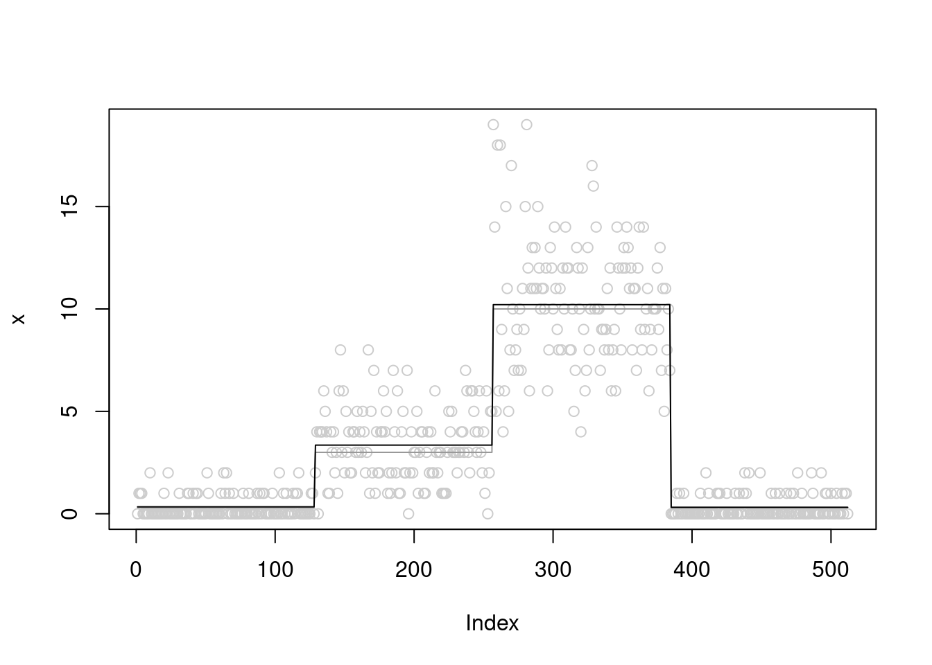
we see that the \(\sigma^2\) converges to 0.
plot(fit$fitted_g$sigma2_trace,type='l')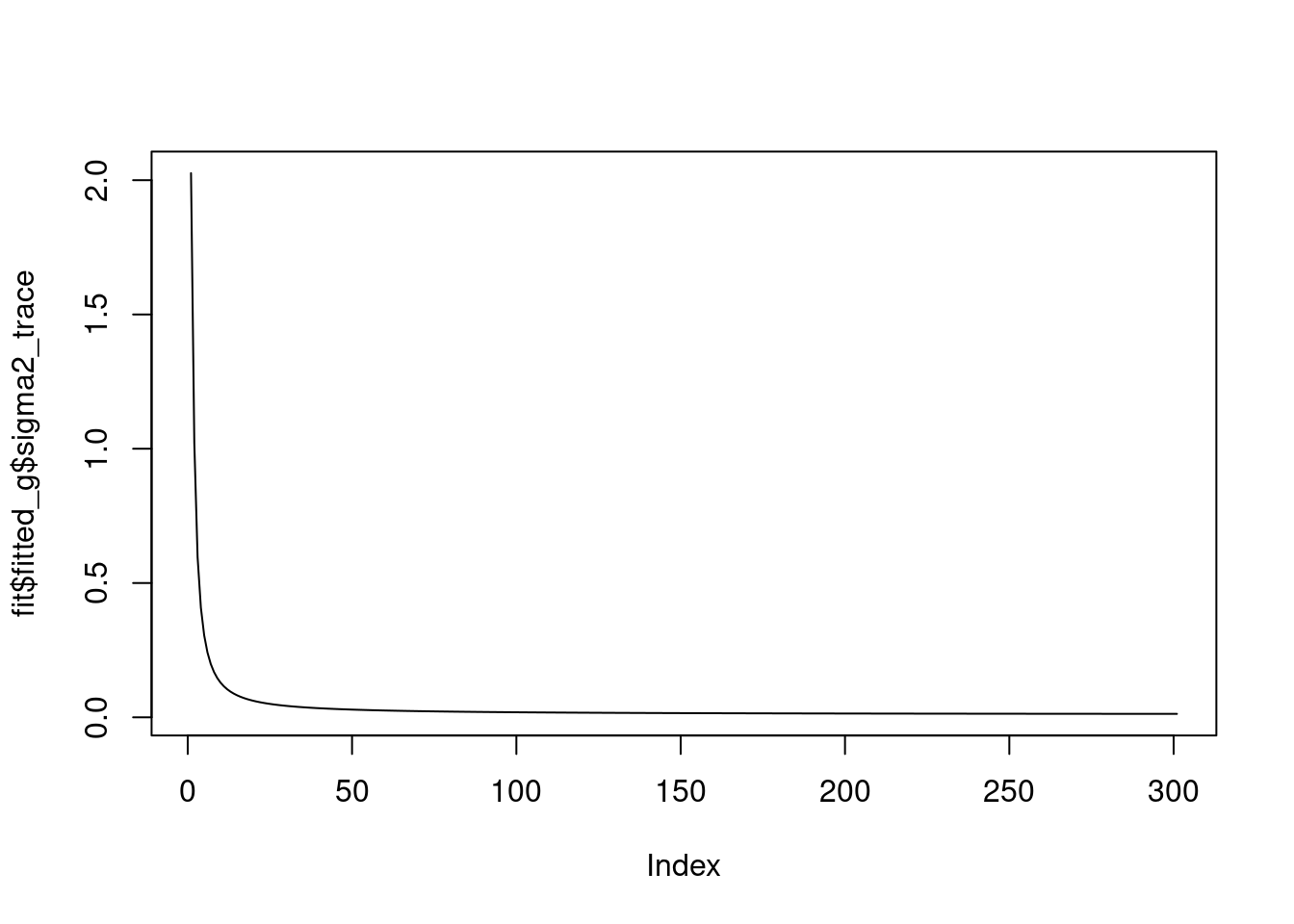
And the priors on wavelet coefficients converge to a point mass. At scale 0 and 1, they are pointmass at non-zero posoitons, and at other scales, they are point mass at 0.
fit$fitted_g$sigma2
[1] 0.01284379
$sigma2_trace
[1] 2.02605584 1.02277958 0.59628740 0.40837161 0.30546363 0.24163674
[7] 0.19882781 0.16848146 0.14604414 0.12889042 0.11541351 0.10458258
[13] 0.09571017 0.08832265 0.08208448 0.07675211 0.07214498 0.06812674
[19] 0.06459263 0.06146100 0.05866736 0.05616011 0.05389755 0.05184561
[25] 0.04997623 0.04826607 0.04669560 0.04524831 0.04391021 0.04266934
[31] 0.04151540 0.04043952 0.03943398 0.03849204 0.03760781 0.03677610
[37] 0.03599232 0.03525240 0.03455273 0.03389009 0.03326157 0.03266458
[43] 0.03209678 0.03155607 0.03104052 0.03054842 0.03007817 0.02962833
[49] 0.02919761 0.02878478 0.02838876 0.02800852 0.02764313 0.02729174
[55] 0.02695354 0.02662780 0.02631385 0.02601105 0.02571881 0.02543659
[61] 0.02516388 0.02490020 0.02464512 0.02439821 0.02415909 0.02392740
[67] 0.02370279 0.02348495 0.02327358 0.02306838 0.02286910 0.02267549
[73] 0.02248730 0.02230431 0.02212631 0.02195311 0.02178450 0.02162032
[79] 0.02146039 0.02130455 0.02115265 0.02100454 0.02086008 0.02071915
[85] 0.02058161 0.02044735 0.02031625 0.02018820 0.02006311 0.01994086
[91] 0.01982138 0.01970456 0.01959032 0.01947859 0.01936927 0.01926229
[97] 0.01915758 0.01905508 0.01895471 0.01885641 0.01876012 0.01866579
[103] 0.01857334 0.01848273 0.01839391 0.01830683 0.01822143 0.01813768
[109] 0.01805552 0.01797491 0.01789581 0.01781818 0.01774199 0.01766719
[115] 0.01759375 0.01752163 0.01745080 0.01738122 0.01731288 0.01724572
[121] 0.01717974 0.01711489 0.01705115 0.01698849 0.01692689 0.01686632
[127] 0.01680676 0.01674818 0.01669057 0.01663390 0.01657814 0.01652328
[133] 0.01646931 0.01641618 0.01636390 0.01631244 0.01626178 0.01621191
[139] 0.01616281 0.01611446 0.01606685 0.01601996 0.01597377 0.01592828
[145] 0.01588347 0.01583932 0.01579582 0.01575295 0.01571072 0.01566909
[151] 0.01562807 0.01558763 0.01554777 0.01550848 0.01546974 0.01543155
[157] 0.01539389 0.01535675 0.01532013 0.01528402 0.01524840 0.01521327
[163] 0.01517861 0.01514442 0.01511070 0.01507742 0.01504459 0.01501220
[169] 0.01498023 0.01494869 0.01491756 0.01488683 0.01485651 0.01482657
[175] 0.01479703 0.01476786 0.01473907 0.01471064 0.01468257 0.01465486
[181] 0.01462750 0.01460048 0.01457379 0.01454744 0.01452142 0.01449571
[187] 0.01447033 0.01444525 0.01442048 0.01439601 0.01437184 0.01434796
[193] 0.01432437 0.01430106 0.01427802 0.01425527 0.01423278 0.01421056
[199] 0.01418860 0.01416690 0.01414545 0.01412426 0.01410331 0.01408260
[205] 0.01406213 0.01404190 0.01402190 0.01400214 0.01398259 0.01396327
[211] 0.01394417 0.01392528 0.01390661 0.01388815 0.01386989 0.01385184
[217] 0.01383399 0.01381634 0.01379888 0.01378162 0.01376455 0.01374766
[223] 0.01373096 0.01371445 0.01369811 0.01368195 0.01366597 0.01365016
[229] 0.01363452 0.01361905 0.01360374 0.01358860 0.01357362 0.01355881
[235] 0.01354414 0.01352964 0.01351528 0.01350108 0.01348703 0.01347313
[241] 0.01345937 0.01344576 0.01343229 0.01341895 0.01340576 0.01339270
[247] 0.01337978 0.01336699 0.01335434 0.01334181 0.01332941 0.01331714
[253] 0.01330500 0.01329298 0.01328108 0.01326930 0.01325764 0.01324610
[259] 0.01323467 0.01322336 0.01321216 0.01320108 0.01319010 0.01317924
[265] 0.01316848 0.01315784 0.01314729 0.01313685 0.01312652 0.01311629
[271] 0.01310615 0.01309612 0.01308619 0.01307635 0.01306661 0.01305696
[277] 0.01304741 0.01303795 0.01302859 0.01301931 0.01301012 0.01300103
[283] 0.01299202 0.01298309 0.01297426 0.01296551 0.01295684 0.01294825
[289] 0.01293975 0.01293133 0.01292299 0.01291472 0.01290654 0.01289843
[295] 0.01289041 0.01288245 0.01287457 0.01286677 0.01285904 0.01285138
[301] 0.01284379
$g
$g[[1]]
$pi
[1] 0 0 1 0
$mean
[1] 0 0 0 0
$sd
[1] 0.000000 2.465394 5.512789 11.297855
attr(,"class")
[1] "normalmix"
attr(,"row.names")
[1] 1 2 3 4
$g[[2]]
$pi
[1] 0 0 0 0 1
$mean
[1] 0 0 0 0 0
$sd
[1] 0.000000 2.465394 5.512789 11.297855 22.729810
attr(,"class")
[1] "normalmix"
attr(,"row.names")
[1] 1 2 3 4 5
$g[[3]]
$pi
[1] 1 0 0
$mean
[1] 0 0 0
$sd
[1] 0.0000000 0.9160894 1.4233959
attr(,"class")
[1] "normalmix"
attr(,"row.names")
[1] 1 2 3
$g[[4]]
$pi
[1] 1 0 0
$mean
[1] 0 0 0
$sd
[1] 0.0000000 0.9160894 1.4233959
attr(,"class")
[1] "normalmix"
attr(,"row.names")
[1] 1 2 3
$g[[5]]
$pi
[1] 1 0 0
$mean
[1] 0 0 0
$sd
[1] 0.0000000 0.9160894 1.4233959
attr(,"class")
[1] "normalmix"
attr(,"row.names")
[1] 1 2 3
$g[[6]]
$pi
[1] 1 0 0
$mean
[1] 0 0 0
$sd
[1] 0.0000000 0.9160894 1.4233959
attr(,"class")
[1] "normalmix"
attr(,"row.names")
[1] 1 2 3
$g[[7]]
$pi
[1] 1 0 0
$mean
[1] 0 0 0
$sd
[1] 0.0000000 0.9183661 1.4275424
attr(,"class")
[1] "normalmix"
attr(,"row.names")
[1] 1 2 3
$g[[8]]
$pi
[1] 1 0 0
$mean
[1] 0 0 0
$sd
[1] 0.0000000 0.9160894 1.4233959
attr(,"class")
[1] "normalmix"
attr(,"row.names")
[1] 1 2 3
$g[[9]]
$pi
[1] 1 0 0
$mean
[1] 0 0 0
$sd
[1] 0.000000 1.036569 1.648872
attr(,"class")
[1] "normalmix"
attr(,"row.names")
[1] 1 2 3The ELBO is
fit$elbo[1] -1037.525Let’s try to initialize at a different value and let it get stuck at a local optimum. In this case,
fit = pois_smooth_split(x,maxiter=300,verbose = T,tol=1e-10,m_init=rep(mean(x),n),sigma2_init = 0.01)[1] "Done iter 10 obj = -1495.02400858245"
[1] "Done iter 20 obj = -1495.00044452096"we see that the \(\sigma^2\) converges to 2.
plot(fit$fitted_g$sigma2_trace,type='l')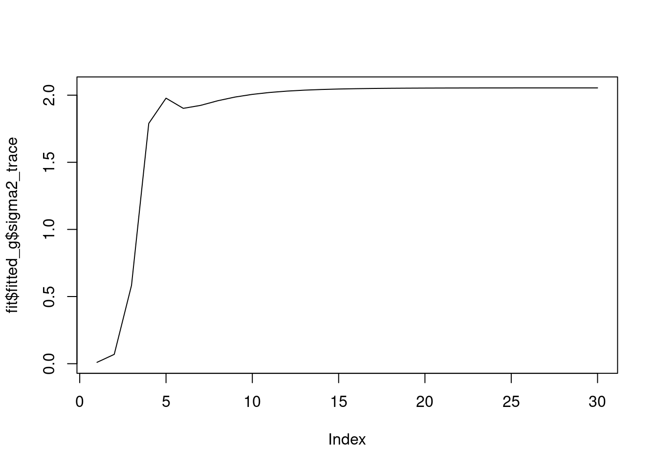
And the priors on wavelet coefficients converge to a point mass at 0.
fit$fitted_g$sigma2
[1] 2.054209
$sigma2_trace
[1] 0.0100000 0.0695137 0.5832216 1.7897822 1.9776397 1.9018849 1.9239050
[8] 1.9586004 1.9860673 2.0059708 2.0201441 2.0301867 2.0372861 2.0422932
[15] 2.0458265 2.0483180 2.0500738 2.0513106 2.0521816 2.0527948 2.0532264
[22] 2.0535302 2.0537441 2.0538945 2.0540004 2.0540750 2.0541274 2.0541643
[29] 2.0541903 2.0542085
$g
$g[[1]]
$pi
[1] 1 0 0
$mean
[1] 0 0 0
$sd
[1] 0.00000000 0.06435943 0.10000000
attr(,"class")
[1] "normalmix"
attr(,"row.names")
[1] 1 2 3
$g[[2]]
$pi
[1] 1 0 0
$mean
[1] 0 0 0
$sd
[1] 0.00000000 0.06435943 0.10000000
attr(,"class")
[1] "normalmix"
attr(,"row.names")
[1] 1 2 3
$g[[3]]
$pi
[1] 1 0 0
$mean
[1] 0 0 0
$sd
[1] 0.00000000 0.06435943 0.10000000
attr(,"class")
[1] "normalmix"
attr(,"row.names")
[1] 1 2 3
$g[[4]]
$pi
[1] 1 0 0
$mean
[1] 0 0 0
$sd
[1] 0.00000000 0.06435943 0.10000000
attr(,"class")
[1] "normalmix"
attr(,"row.names")
[1] 1 2 3
$g[[5]]
$pi
[1] 1 0 0
$mean
[1] 0 0 0
$sd
[1] 0.00000000 0.06435943 0.10000000
attr(,"class")
[1] "normalmix"
attr(,"row.names")
[1] 1 2 3
$g[[6]]
$pi
[1] 1 0 0
$mean
[1] 0 0 0
$sd
[1] 0.00000000 0.06435943 0.10000000
attr(,"class")
[1] "normalmix"
attr(,"row.names")
[1] 1 2 3
$g[[7]]
$pi
[1] 1 0 0
$mean
[1] 0 0 0
$sd
[1] 0.00000000 0.06435943 0.10000000
attr(,"class")
[1] "normalmix"
attr(,"row.names")
[1] 1 2 3
$g[[8]]
$pi
[1] 1 0 0
$mean
[1] 0 0 0
$sd
[1] 0.00000000 0.06435943 0.10000000
attr(,"class")
[1] "normalmix"
attr(,"row.names")
[1] 1 2 3
$g[[9]]
$pi
[1] 1 0 0
$mean
[1] 0 0 0
$sd
[1] 0.00000000 0.06435943 0.10000000
attr(,"class")
[1] "normalmix"
attr(,"row.names")
[1] 1 2 3The ELBO is
fit$elbo[1] -1495A simple curve
We use non-haar wavelet here. THe function is spike.
set.seed(12345)
n=2^9
count_size = 20
sigma=0.5
t = seq(0,1,length.out = n)
b = smashrgen:::spike.f(t)
b = b/(max(b)/count_size)
x = rpois(n,exp(log(b)+rnorm(n,sd=sigma)))
plot(x,col='grey80')
lines(b,col='grey50')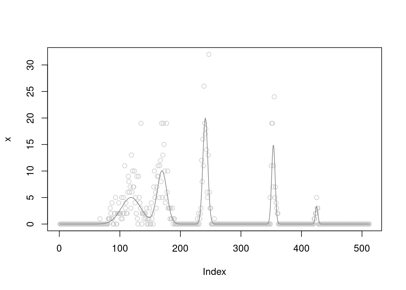
fit = pois_smooth_split(x,maxiter=300,verbose = T,tol=1e-10,filter.number = 8)[1] "Done iter 10 obj = -743.002062920863"
[1] "Done iter 20 obj = -735.434818580334"
[1] "Done iter 30 obj = -733.787084937347"
[1] "Done iter 40 obj = -733.177171521856"
[1] "Done iter 50 obj = -732.849817379526"
[1] "Done iter 60 obj = -732.62896781191"
[1] "Done iter 70 obj = -732.461913972196"
[1] "Done iter 80 obj = -732.328794150765"
[1] "Done iter 90 obj = -732.220113985061"
[1] "Done iter 100 obj = -732.130279053868"
[1] "Done iter 110 obj = -732.055480559091"
[1] "Done iter 120 obj = -731.992898773365"
[1] "Done iter 130 obj = -731.940349052054"
[1] "Done iter 140 obj = -731.896095504677"
[1] "Done iter 150 obj = -731.858737820622"
[1] "Done iter 160 obj = -731.827135135782"
[1] "Done iter 170 obj = -731.800351323234"
[1] "Done iter 180 obj = -731.777614021518"
[1] "Done iter 190 obj = -731.758283130143"
[1] "Done iter 200 obj = -731.741826150613"
[1] "Done iter 210 obj = -731.727798641114"
[1] "Done iter 220 obj = -731.715828576806"
[1] "Done iter 230 obj = -731.705603740449"
[1] "Done iter 240 obj = -731.696861492824"
[1] "Done iter 250 obj = -731.689380429482"
[1] "Done iter 260 obj = -731.682973544411"
[1] "Done iter 270 obj = -731.677482605196"
[1] "Done iter 280 obj = -731.672773507776"
[1] "Done iter 290 obj = -731.668732427169"
[1] "Done iter 300 obj = -731.665262617926"plot(x,col='grey80')
lines(b,col='grey60')
lines(fit$posterior$mean_smooth,col=4)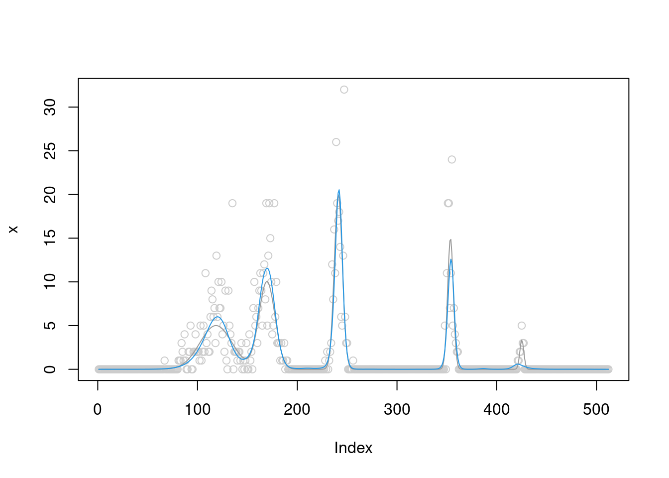
The \(\sigma^2\) converges to 0.4.
plot(fit$fitted_g$sigma2_trace)
fit$fitted_g$sigma2[1] 0.3774314And the priors on wavelet coefficients converge to a point mass at finer level.
At scale 5 and 2, the prior converges to a mixture of two normals.
At scale 0 and 1, they are point-mass at non-zero positions.
fit$fitted_g$sigma2
[1] 0.3774314
$sigma2_trace
[1] 4.9656857 3.2404075 2.2560725 1.7392224 1.4245901 1.2127665 1.0612812
[8] 0.9481292 0.8607650 0.7915536 0.7355879 0.6895700 0.6512017 0.6188339
[15] 0.5912535 0.5675489 0.5470225 0.5291314 0.5134468 0.4996261 0.4873920
[22] 0.4765182 0.4668176 0.4581351 0.4503405 0.4433238 0.4369917 0.4312647
[29] 0.4260742 0.4213610 0.4170739 0.4131683 0.4096051 0.4063500 0.4033726
[36] 0.4006465 0.3981477 0.3958553 0.3937505 0.3918164 0.3900381 0.3884019
[43] 0.3868958 0.3855088 0.3842309 0.3830531 0.3819674 0.3809663 0.3800431
[50] 0.3791916 0.3784064 0.3776822 0.3770144 0.3763987 0.3758313 0.3753085
[57] 0.3748269 0.3743837 0.3739759 0.3736011 0.3732567 0.3729407 0.3726510
[64] 0.3723858 0.3721433 0.3719219 0.3717201 0.3715366 0.3713701 0.3712194
[71] 0.3710834 0.3709612 0.3708517 0.3707540 0.3706674 0.3705912 0.3705245
[78] 0.3704667 0.3704173 0.3703756 0.3703412 0.3703135 0.3702920 0.3702763
[85] 0.3702661 0.3702609 0.3702605 0.3702644 0.3702723 0.3702840 0.3702993
[92] 0.3703178 0.3703393 0.3703636 0.3703905 0.3704198 0.3704513 0.3704849
[99] 0.3705205 0.3705577 0.3705966 0.3706370 0.3706787 0.3707217 0.3707659
[106] 0.3708111 0.3708573 0.3709043 0.3709522 0.3710007 0.3710499 0.3710997
[113] 0.3711500 0.3712008 0.3712520 0.3713035 0.3713553 0.3714074 0.3714597
[120] 0.3715122 0.3715649 0.3716176 0.3716705 0.3717233 0.3717763 0.3718292
[127] 0.3718820 0.3719349 0.3719876 0.3720403 0.3720928 0.3721453 0.3721975
[134] 0.3722497 0.3723016 0.3723534 0.3724050 0.3724563 0.3725075 0.3725584
[141] 0.3726091 0.3726596 0.3727098 0.3727597 0.3728094 0.3728588 0.3729080
[148] 0.3729569 0.3730055 0.3730538 0.3731018 0.3731495 0.3731969 0.3732440
[155] 0.3732909 0.3733374 0.3733836 0.3734296 0.3734752 0.3735205 0.3735655
[162] 0.3736102 0.3736546 0.3736987 0.3737424 0.3737859 0.3738291 0.3738719
[169] 0.3739145 0.3739567 0.3739986 0.3740403 0.3740816 0.3741226 0.3741633
[176] 0.3742037 0.3742439 0.3742837 0.3743232 0.3743624 0.3744014 0.3744400
[183] 0.3744784 0.3745164 0.3745542 0.3745917 0.3746289 0.3746658 0.3747025
[190] 0.3747388 0.3747749 0.3748107 0.3748462 0.3748815 0.3749165 0.3749512
[197] 0.3749856 0.3750198 0.3750537 0.3750874 0.3751208 0.3751539 0.3751868
[204] 0.3752194 0.3752518 0.3752839 0.3753158 0.3753474 0.3753788 0.3754100
[211] 0.3754408 0.3754715 0.3755019 0.3755321 0.3755620 0.3755918 0.3756212
[218] 0.3756505 0.3756795 0.3757083 0.3757369 0.3757652 0.3757934 0.3758213
[225] 0.3758490 0.3758764 0.3759037 0.3759308 0.3759576 0.3759842 0.3760107
[232] 0.3760369 0.3760629 0.3760887 0.3761143 0.3761397 0.3761649 0.3761900
[239] 0.3762148 0.3762394 0.3762639 0.3762881 0.3763122 0.3763360 0.3763597
[246] 0.3763832 0.3764066 0.3764297 0.3764527 0.3764754 0.3764980 0.3765205
[253] 0.3765427 0.3765648 0.3765867 0.3766085 0.3766300 0.3766514 0.3766727
[260] 0.3766938 0.3767147 0.3767354 0.3767560 0.3767765 0.3767967 0.3768168
[267] 0.3768368 0.3768566 0.3768763 0.3768958 0.3769151 0.3769343 0.3769534
[274] 0.3769723 0.3769911 0.3770097 0.3770282 0.3770465 0.3770647 0.3770827
[281] 0.3771006 0.3771184 0.3771361 0.3771536 0.3771709 0.3771882 0.3772053
[288] 0.3772222 0.3772391 0.3772558 0.3772724 0.3772888 0.3773051 0.3773214
[295] 0.3773374 0.3773534 0.3773692 0.3773849 0.3774005 0.3774160 0.3774314
$g
$g[[1]]
$pi
[1] 1 0 0
$mean
[1] 0 0 0
$sd
[1] 0.000000 1.434174 2.228382
attr(,"class")
[1] "normalmix"
attr(,"row.names")
[1] 1 2 3
$g[[2]]
$pi
[1] 0.4911003 0.0000000 0.0000000 0.0000000 0.5088997
$mean
[1] 0 0 0 0 0
$sd
[1] 0.000000 3.859671 8.630486 17.687233 35.584405
attr(,"class")
[1] "normalmix"
attr(,"row.names")
[1] 1 2 3 4 5
$g[[3]]
$pi
[1] 0 1 0
$mean
[1] 0 0 0
$sd
[1] 0.000000 2.334316 4.108222
attr(,"class")
[1] "normalmix"
attr(,"row.names")
[1] 1 2 3
$g[[4]]
$pi
[1] 0.3216471 0.0000000 0.6783529 0.0000000
$mean
[1] 0 0 0 0
$sd
[1] 0.000000 3.859671 8.630486 17.687233
attr(,"class")
[1] "normalmix"
attr(,"row.names")
[1] 1 2 3 4
$g[[5]]
$pi
[1] 0.5937845 0.0000000 0.4062155 0.0000000
$mean
[1] 0 0 0 0
$sd
[1] 0.000000 3.859671 8.630486 17.687233
attr(,"class")
[1] "normalmix"
attr(,"row.names")
[1] 1 2 3 4
$g[[6]]
$pi
[1] 1 0 0
$mean
[1] 0 0 0
$sd
[1] 0.000000 2.404843 4.278086
attr(,"class")
[1] "normalmix"
attr(,"row.names")
[1] 1 2 3
$g[[7]]
$pi
[1] 1 0 0
$mean
[1] 0 0 0
$sd
[1] 0.000000 1.561357 2.464244
attr(,"class")
[1] "normalmix"
attr(,"row.names")
[1] 1 2 3
$g[[8]]
$pi
[1] 1 0 0
$mean
[1] 0 0 0
$sd
[1] 0.000000 1.434174 2.228382
attr(,"class")
[1] "normalmix"
attr(,"row.names")
[1] 1 2 3
$g[[9]]
$pi
[1] 1 0 0
$mean
[1] 0 0 0
$sd
[1] 0.000000 1.739671 2.810241
attr(,"class")
[1] "normalmix"
attr(,"row.names")
[1] 1 2 3The ELBO is
fit$elbo[1] -731.6653Let’s try to initialize at a different value and let it get stuck at a local optimum. In this case,
fit = pois_smooth_split(x,maxiter=300,verbose = T,tol=1e-10,m_init=rep(mean(x),n),sigma2_init = 0.01)[1] "Done iter 10 obj = -1456.42959848876"
[1] "Done iter 20 obj = -999.62287908242"
[1] "Done iter 30 obj = -992.985255538695"
[1] "Done iter 40 obj = -992.771343548446"
[1] "Done iter 50 obj = -992.763253762118"
[1] "Done iter 60 obj = -992.762937263367"
[1] "Done iter 70 obj = -992.762924848657"plot(x,col='grey80')
lines(b,col='grey60')
lines(fit$posterior$mean_smooth,col=4)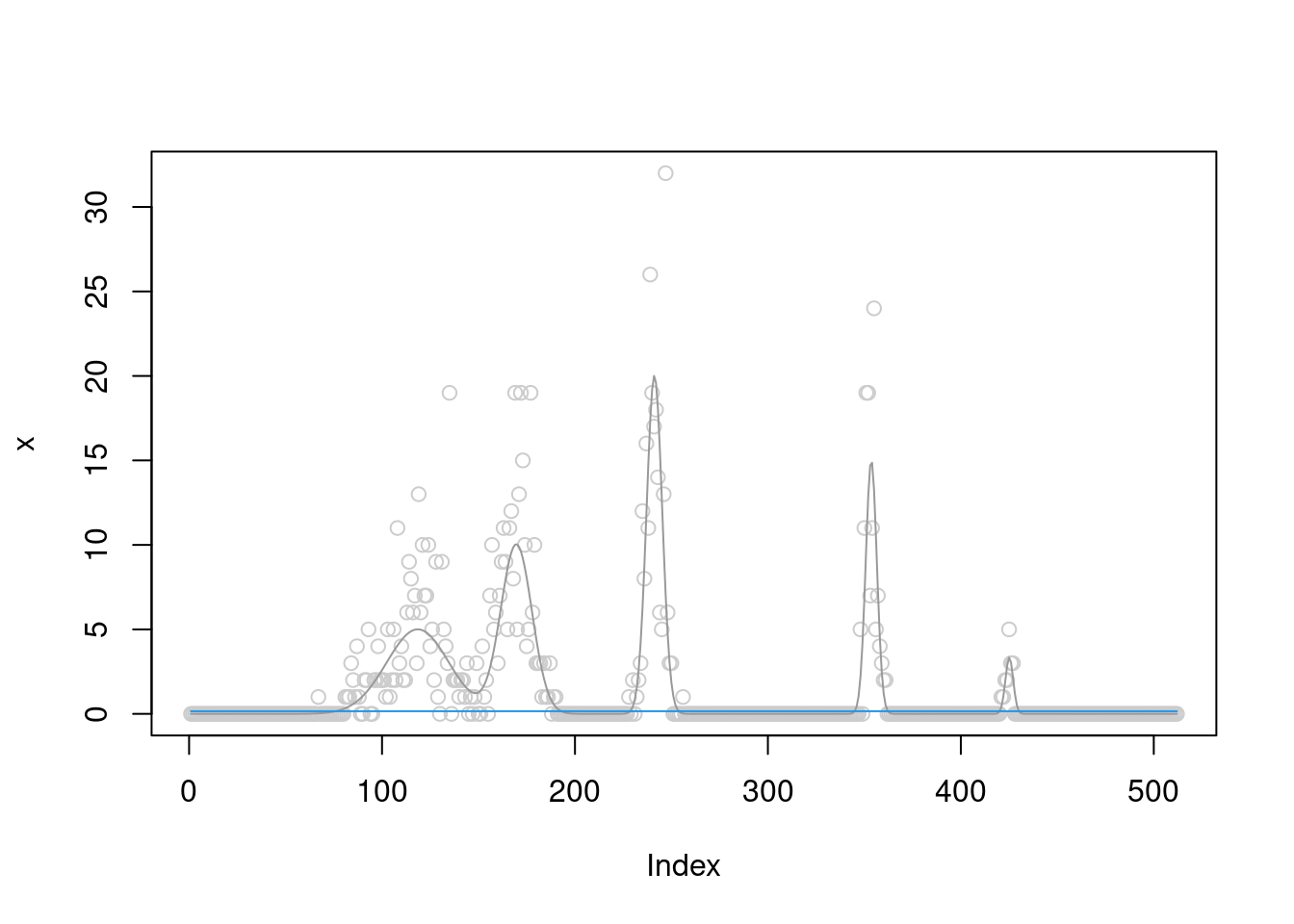
The \(\sigma^2\) converges to 5.47.
plot(fit$fitted_g$sigma2_trace)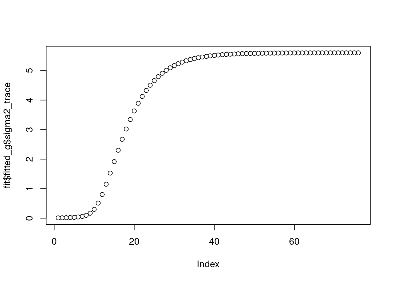
fit$fitted_g$sigma2[1] 5.600328And the priors on wavelet coefficients converge to a point mass at 0.
fit$fitted_g$sigma2
[1] 5.600328
$sigma2_trace
[1] 0.01000000 0.01225251 0.01541753 0.02005395 0.02719408 0.03885680
[7] 0.05918851 0.09681917 0.16837188 0.29886140 0.51008592 0.80148880
[13] 1.14938043 1.52691675 1.91519747 2.30052627 2.67172657 3.02041082
[19] 3.34136807 3.63217701 3.89247318 4.12325268 4.32632311 4.50395386
[25] 4.65859223 4.79268884 4.90860056 5.00852990 5.09449327 5.16830908
[31] 5.23159865 5.28579486 5.33215539 5.37177807 5.40561697 5.43449824
[37] 5.45913518 5.48014212 5.49804714 5.51330339 5.52628735 5.53733691
[43] 5.54674958 5.55476708 5.56159483 5.56740830 5.57235739 5.57657004
[49] 5.58015542 5.58320663 5.58580303 5.58801227 5.58989196 5.59149117
[55] 5.59285171 5.59400914 5.59499375 5.59583133 5.59654382 5.59714989
[61] 5.59766542 5.59810393 5.59847693 5.59879419 5.59906406 5.59929359
[67] 5.59948883 5.59965489 5.59979614 5.59991627 5.60001846 5.60010537
[73] 5.60017929 5.60024216 5.60029564 5.60032834
$g
$g[[1]]
$pi
[1] 1 0 0
$mean
[1] 0 0 0
$sd
[1] 0.00000000 0.06435943 0.10000000
attr(,"class")
[1] "normalmix"
attr(,"row.names")
[1] 1 2 3
$g[[2]]
$pi
[1] 1 0 0
$mean
[1] 0 0 0
$sd
[1] 0.00000000 0.06435943 0.10000000
attr(,"class")
[1] "normalmix"
attr(,"row.names")
[1] 1 2 3
$g[[3]]
$pi
[1] 1 0 0
$mean
[1] 0 0 0
$sd
[1] 0.00000000 0.06435943 0.10000000
attr(,"class")
[1] "normalmix"
attr(,"row.names")
[1] 1 2 3
$g[[4]]
$pi
[1] 1 0 0
$mean
[1] 0 0 0
$sd
[1] 0.00000000 0.06435943 0.10000000
attr(,"class")
[1] "normalmix"
attr(,"row.names")
[1] 1 2 3
$g[[5]]
$pi
[1] 1 0 0
$mean
[1] 0 0 0
$sd
[1] 0.00000000 0.06435943 0.10000000
attr(,"class")
[1] "normalmix"
attr(,"row.names")
[1] 1 2 3
$g[[6]]
$pi
[1] 1 0 0
$mean
[1] 0 0 0
$sd
[1] 0.00000000 0.06435943 0.10000000
attr(,"class")
[1] "normalmix"
attr(,"row.names")
[1] 1 2 3
$g[[7]]
$pi
[1] 1 0 0
$mean
[1] 0 0 0
$sd
[1] 0.00000000 0.06435943 0.10000000
attr(,"class")
[1] "normalmix"
attr(,"row.names")
[1] 1 2 3
$g[[8]]
$pi
[1] 1 0 0
$mean
[1] 0 0 0
$sd
[1] 0.00000000 0.06435943 0.10000000
attr(,"class")
[1] "normalmix"
attr(,"row.names")
[1] 1 2 3
$g[[9]]
$pi
[1] 1 0 0
$mean
[1] 0 0 0
$sd
[1] 0.00000000 0.06435943 0.10000000
attr(,"class")
[1] "normalmix"
attr(,"row.names")
[1] 1 2 3The ELBO is
fit$elbo[1] -992.7629What if I still use a Haar wavelet?
fit = pois_smooth_split(x,maxiter=300,verbose = T,tol=1e-10,filter.number = 1)[1] "Done iter 10 obj = -786.178806533818"
[1] "Done iter 20 obj = -781.632658171641"
[1] "Done iter 30 obj = -781.031816096536"
[1] "Done iter 40 obj = -780.848198431276"
[1] "Done iter 50 obj = -780.748519549505"
[1] "Done iter 60 obj = -780.681900966256"
[1] "Done iter 70 obj = -780.634625231853"
[1] "Done iter 80 obj = -780.600333815418"
[1] "Done iter 90 obj = -780.575169892547"
[1] "Done iter 100 obj = -780.556555221732"
[1] "Done iter 110 obj = -780.542698495885"
[1] "Done iter 120 obj = -780.532329821332"
[1] "Done iter 130 obj = -780.524536825411"
[1] "Done iter 140 obj = -780.518657297232"
[1] "Done iter 150 obj = -780.514206604585"
[1] "Done iter 160 obj = -780.510827603781"
[1] "Done iter 170 obj = -780.508255536755"
[1] "Done iter 180 obj = -780.506293124256"
[1] "Done iter 190 obj = -780.504792709038"
[1] "Done iter 200 obj = -780.50364333945"
[1] "Done iter 210 obj = -780.502761354724"
[1] "Done iter 220 obj = -780.502083476753"
[1] "Done iter 230 obj = -780.501561711369"
[1] "Done iter 240 obj = -780.50115956577"
[1] "Done iter 250 obj = -780.500849229557"
[1] "Done iter 260 obj = -780.500609465407"
[1] "Done iter 270 obj = -780.500424025003"
[1] "Done iter 280 obj = -780.500280455584"
[1] "Done iter 290 obj = -780.500169198135"
[1] "Done iter 300 obj = -780.500082904157"plot(x,col='grey80')
lines(b,col='grey60')
lines(fit$posterior$mean_smooth,col=4)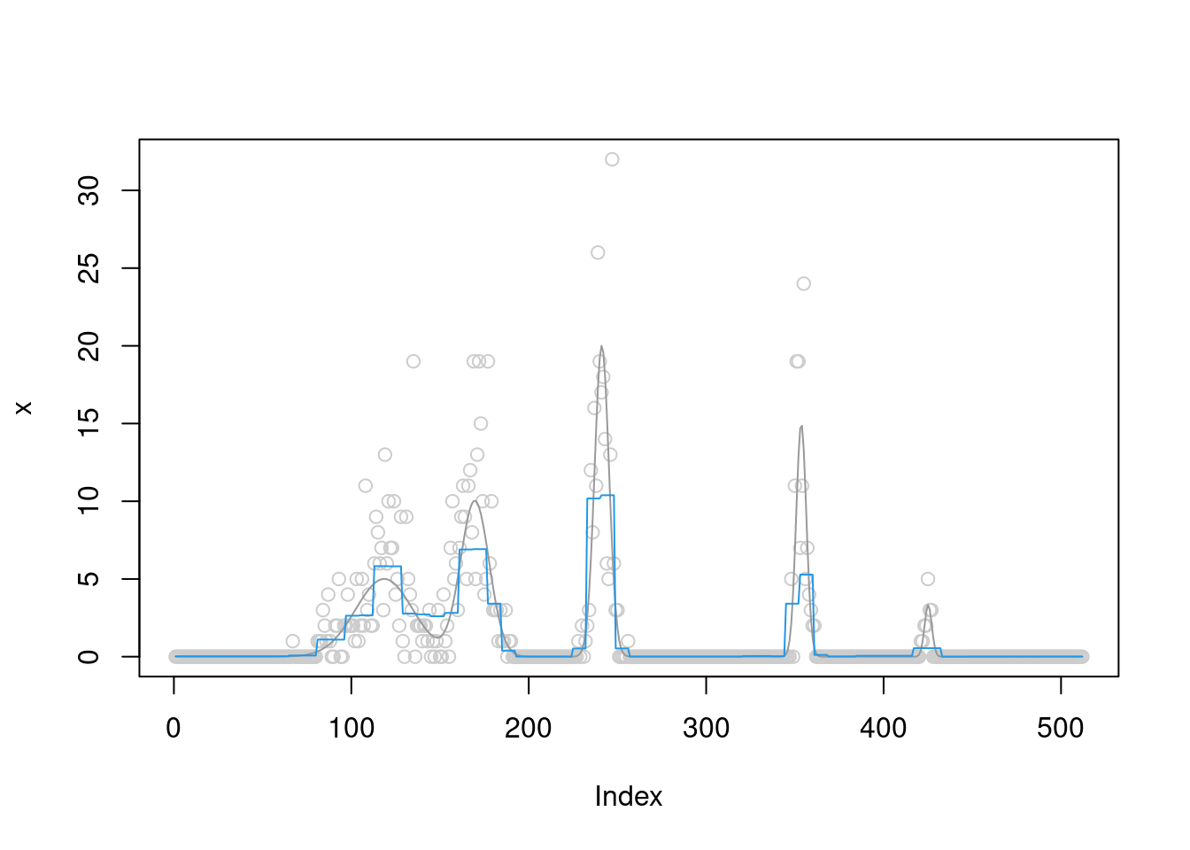
The \(\sigma^2\) converges to 0.8.
plot(fit$fitted_g$sigma2_trace)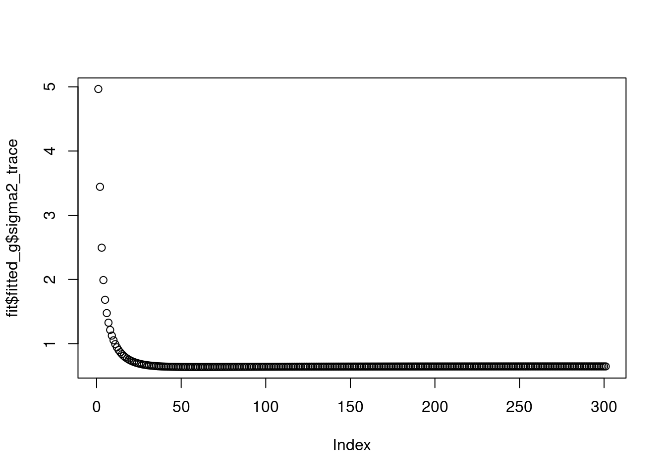
fit$fitted_g$sigma2[1] 0.6458129The prior does not converge to point-mass at scale 4,5,6.
The ELBO is
fit$elbo[1] -780.5001Observations
It seems that for the smoothing problem:
If \(g\) goes to pointmass at 0, then estimated \(\sigma^2\) is large. This is the same as in Poisson mean problem.
If \(g\) goes to non-point mass(In wavelet case, some of the them maybe point mass, but at least one of them is not), then \(\sigma^2\) can converge to smaller value, but not 0.
If \(g\) goes to pointmass’s, but not all at 0. This corresponding to the first example. Then in this case \(\sigma^2\) seems to be able to converge to 0. And apparently the estimated curve is close to the true one, as shown in plot.
sessionInfo()R version 4.2.2 Patched (2022-11-10 r83330)
Platform: x86_64-pc-linux-gnu (64-bit)
Running under: Ubuntu 22.04.1 LTS
Matrix products: default
BLAS: /usr/lib/x86_64-linux-gnu/openblas-pthread/libblas.so.3
LAPACK: /usr/lib/x86_64-linux-gnu/openblas-pthread/libopenblasp-r0.3.20.so
locale:
[1] LC_CTYPE=en_US.UTF-8 LC_NUMERIC=C
[3] LC_TIME=en_US.UTF-8 LC_COLLATE=en_US.UTF-8
[5] LC_MONETARY=en_US.UTF-8 LC_MESSAGES=en_US.UTF-8
[7] LC_PAPER=en_US.UTF-8 LC_NAME=C
[9] LC_ADDRESS=C LC_TELEPHONE=C
[11] LC_MEASUREMENT=en_US.UTF-8 LC_IDENTIFICATION=C
attached base packages:
[1] stats graphics grDevices utils datasets methods base
other attached packages:
[1] smashrgen_1.1.5 wavethresh_4.7.2 MASS_7.3-58.2 caTools_1.18.2
[5] ashr_2.2-54 smashr_1.3-6 workflowr_1.7.0
loaded via a namespace (and not attached):
[1] httr_1.4.4 sass_0.4.4 jsonlite_1.8.4 splines_4.2.2
[5] foreach_1.5.2 bslib_0.4.2 getPass_0.2-2 horseshoe_0.2.0
[9] highr_0.9 mixsqp_0.3-48 deconvolveR_1.2-1 yaml_2.3.6
[13] ebnm_1.0-11 pillar_1.8.1 lattice_0.20-45 glue_1.6.2
[17] digest_0.6.31 promises_1.2.0.1 colorspace_2.0-3 htmltools_0.5.4
[21] httpuv_1.6.7 Matrix_1.5-3 mr.ash_0.1-87 pkgconfig_2.0.3
[25] invgamma_1.1 scales_1.2.1 processx_3.8.0 whisker_0.4.1
[29] later_1.3.0 git2r_0.30.1 tibble_3.1.8 generics_0.1.3
[33] ggplot2_3.4.0 cachem_1.0.6 cli_3.4.1 survival_3.5-0
[37] magrittr_2.0.3 evaluate_0.19 ps_1.7.2 ebpm_0.0.1.3
[41] fs_1.5.2 fansi_1.0.3 truncnorm_1.0-8 tools_4.2.2
[45] data.table_1.14.6 lifecycle_1.0.3 matrixStats_0.63.0 stringr_1.5.0
[49] trust_0.1-8 munsell_0.5.0 glmnet_4.1-6 irlba_2.3.5.1
[53] callr_3.7.3 compiler_4.2.2 jquerylib_0.1.4 vebpm_0.4.0
[57] rlang_1.0.6 grid_4.2.2 nloptr_2.0.3 iterators_1.0.14
[61] rstudioapi_0.14 bitops_1.0-7 rmarkdown_2.19 codetools_0.2-18
[65] gtable_0.3.1 R6_2.5.1 knitr_1.41 dplyr_1.0.10
[69] fastmap_1.1.0 utf8_1.2.2 rprojroot_2.0.3 shape_1.4.6
[73] stringi_1.7.8 parallel_4.2.2 SQUAREM_2021.1 Rcpp_1.0.9
[77] vctrs_0.5.1 tidyselect_1.2.0 xfun_0.35