run splitting PMF on pbmc data with more iterations
DongyueXie
2023-01-01
Last updated: 2023-01-09
Checks: 7 0
Knit directory: gsmash/
This reproducible R Markdown analysis was created with workflowr (version 1.6.2). The Checks tab describes the reproducibility checks that were applied when the results were created. The Past versions tab lists the development history.
Great! Since the R Markdown file has been committed to the Git repository, you know the exact version of the code that produced these results.
Great job! The global environment was empty. Objects defined in the global environment can affect the analysis in your R Markdown file in unknown ways. For reproduciblity it’s best to always run the code in an empty environment.
The command set.seed(20220606) was run prior to running
the code in the R Markdown file. Setting a seed ensures that any results
that rely on randomness, e.g. subsampling or permutations, are
reproducible.
Great job! Recording the operating system, R version, and package versions is critical for reproducibility.
Nice! There were no cached chunks for this analysis, so you can be confident that you successfully produced the results during this run.
Great job! Using relative paths to the files within your workflowr project makes it easier to run your code on other machines.
Great! You are using Git for version control. Tracking code development and connecting the code version to the results is critical for reproducibility.
The results in this page were generated with repository version 2779b13. See the Past versions tab to see a history of the changes made to the R Markdown and HTML files.
Note that you need to be careful to ensure that all relevant files for
the analysis have been committed to Git prior to generating the results
(you can use wflow_publish or
wflow_git_commit). workflowr only checks the R Markdown
file, but you know if there are other scripts or data files that it
depends on. Below is the status of the Git repository when the results
were generated:
Ignored files:
    Ignored:    .Rhistory
    Ignored:    .Rproj.user/

Untracked files:
    Untracked:  analysis/size_of_sigma2_on_convergence.Rmd

Unstaged changes:
    Modified:   analysis/overdispersed_splitting.Rmd
Note that any generated files, e.g. HTML, png, CSS, etc., are not included in this status report because it is ok for generated content to have uncommitted changes.
These are the previous versions of the repository in which changes were
made to the R Markdown
(analysis/run_PMF_on_pbmc_more_iterations.Rmd) and HTML
(docs/run_PMF_on_pbmc_more_iterations.html) files. If
you’ve configured a remote Git repository (see
?wflow_git_remote), click on the hyperlinks in the table
below to view the files as they were in that past version.
| File | Version | Author | Date | Message |
|---|---|---|---|---|
| Rmd | 2779b13 | DongyueXie | 2023-01-09 | wflow_publish("analysis/run_PMF_on_pbmc_more_iterations.Rmd") |
| html | 42f0de4 | DongyueXie | 2023-01-05 | Build site. |
| Rmd | 25e29e2 | DongyueXie | 2023-01-05 | wflow_publish("analysis/run_PMF_on_pbmc_more_iterations.Rmd") |
Introduction
I have a previous result run the very initial version of the splitting PMF. Now I revise the code and re-run the model. THe main diff is a. run vga 1 iter every big iteration; b. 1000 iterations; c. add 1 dimension each add_greedy attempt.
I set the scaling factors as \(s_{ij} =
\frac{y_{i+}y_{+j}}{y_{++}}\). For comparison, I also fit
flash on transformed count data, as \(\tilde{y}_{ij} =
\log(1+\frac{y_{ij}}{s_{i}}\frac{a}{0.5})\) where \(s_i=\sum_j y_{ij}\), \(a = median(s_{i})\).
library(fastTopics)
library(Matrix)
library(stm)
data(pbmc_facs)
counts <- pbmc_facs$counts
table(pbmc_facs$samples$subpop)
 B cell   CD14+   CD34+ NK cell  T cell
    767     163     687     673    1484
fit = readRDS('/project2/mstephens/dongyue/poisson_mf/pbmc3k/pbmc_splitting_point_normal_vga1.rds')plot(fit$K_trace, ylab='K',xlab='iterations')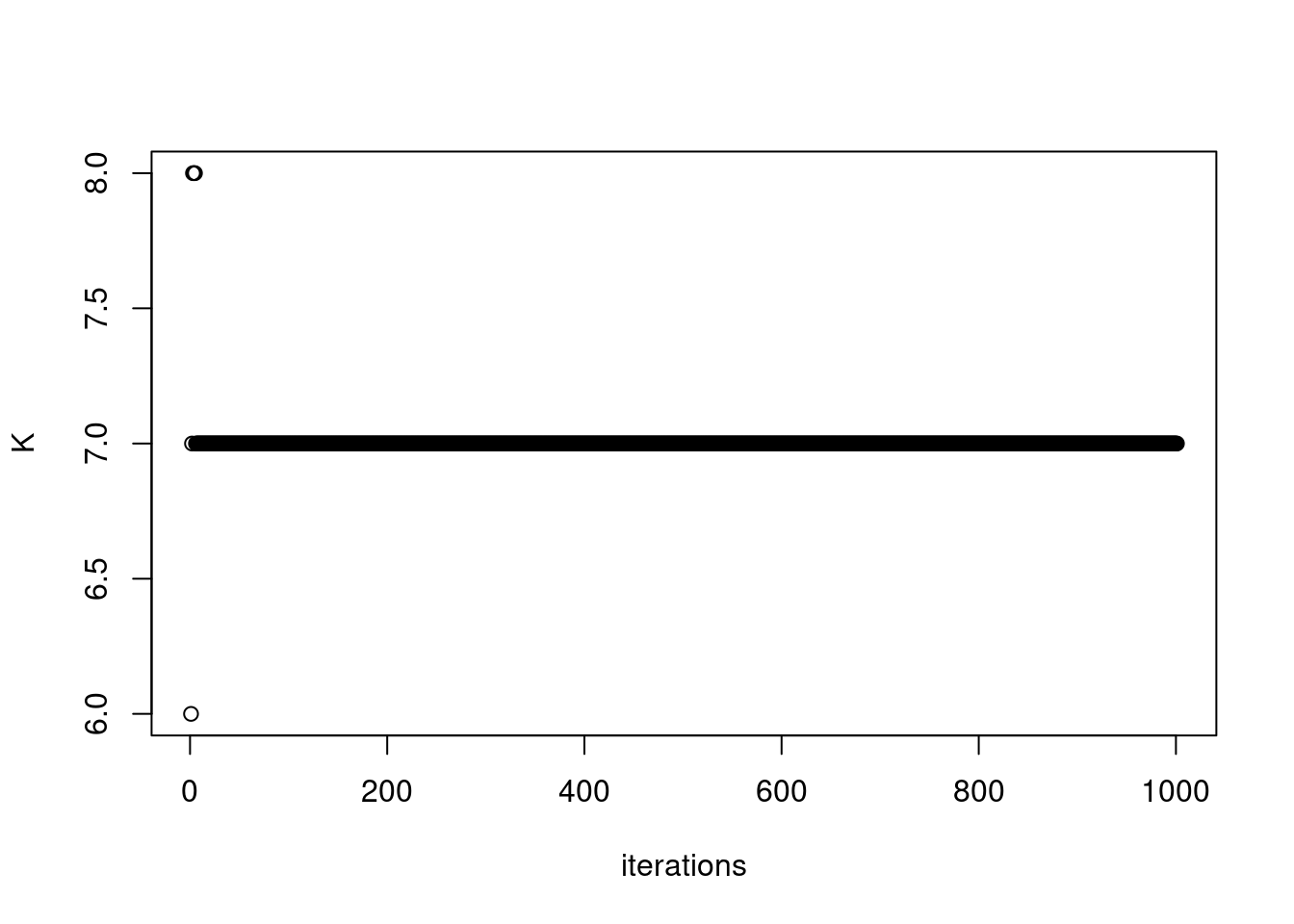
| Version | Author | Date |
|---|---|---|
| 42f0de4 | DongyueXie | 2023-01-05 |
plot(fit$elbo_trace,ylab='elbo',xlab='iterations',type='l')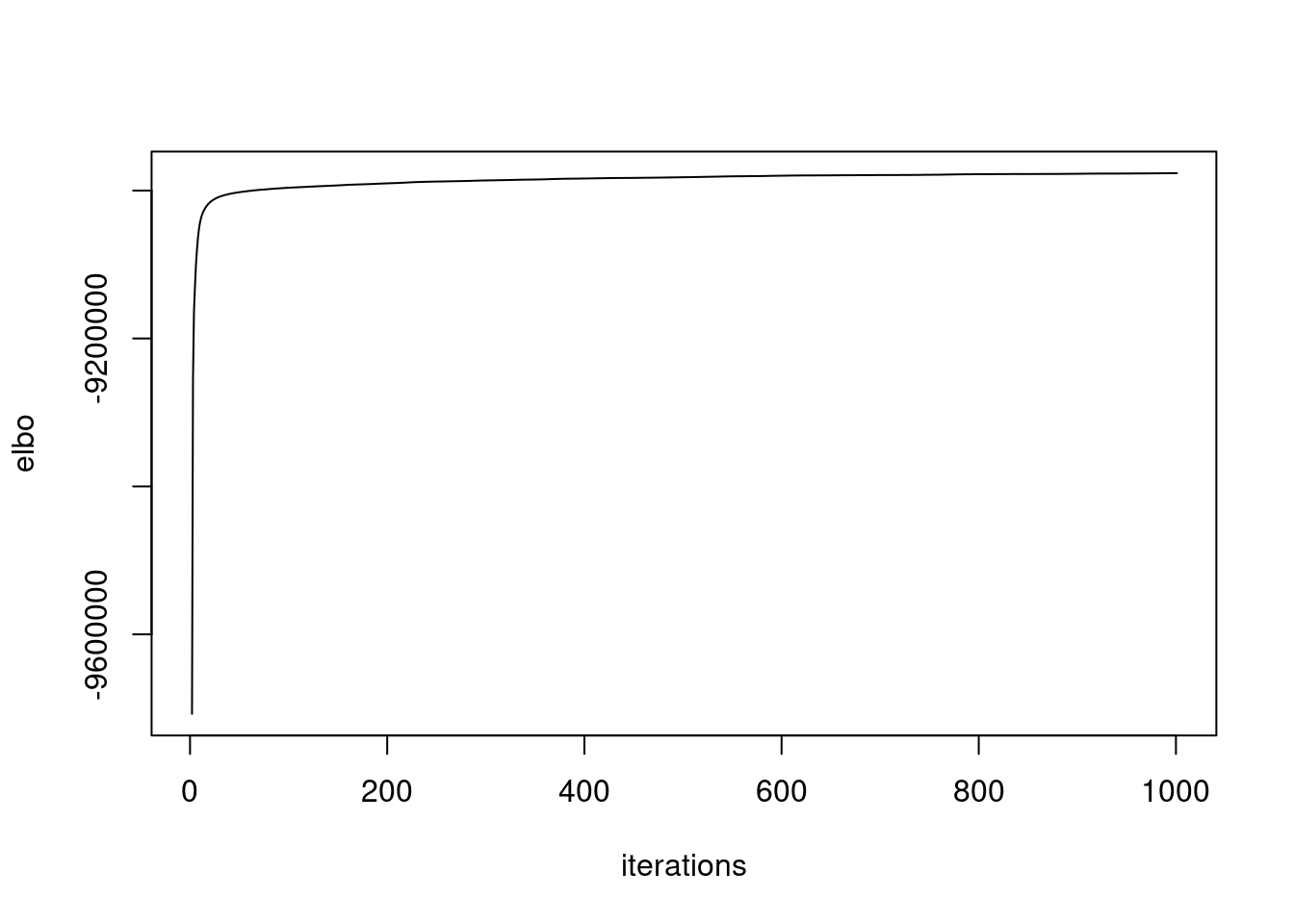
| Version | Author | Date |
|---|---|---|
| 42f0de4 | DongyueXie | 2023-01-05 |
plot(colSums(counts/c(rowSums(counts)))/dim(counts)[1],fit$sigma2,xlab='gene mean count(after library size adjustment)')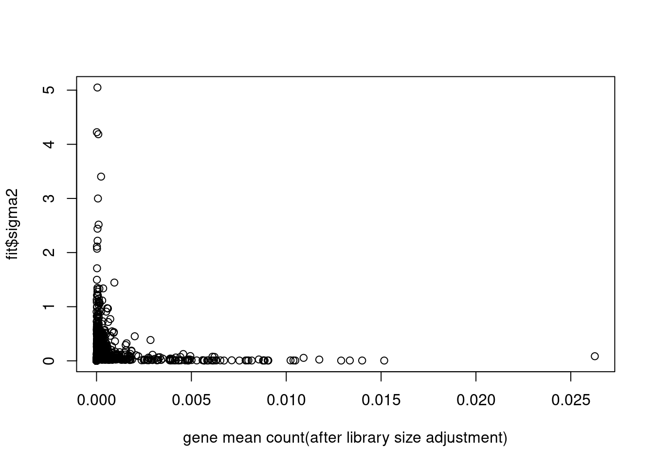
| Version | Author | Date |
|---|---|---|
| 42f0de4 | DongyueXie | 2023-01-05 |
plot(colSums(counts==0)/dim(counts)[1],fit$sigma2,xlab='sparsity')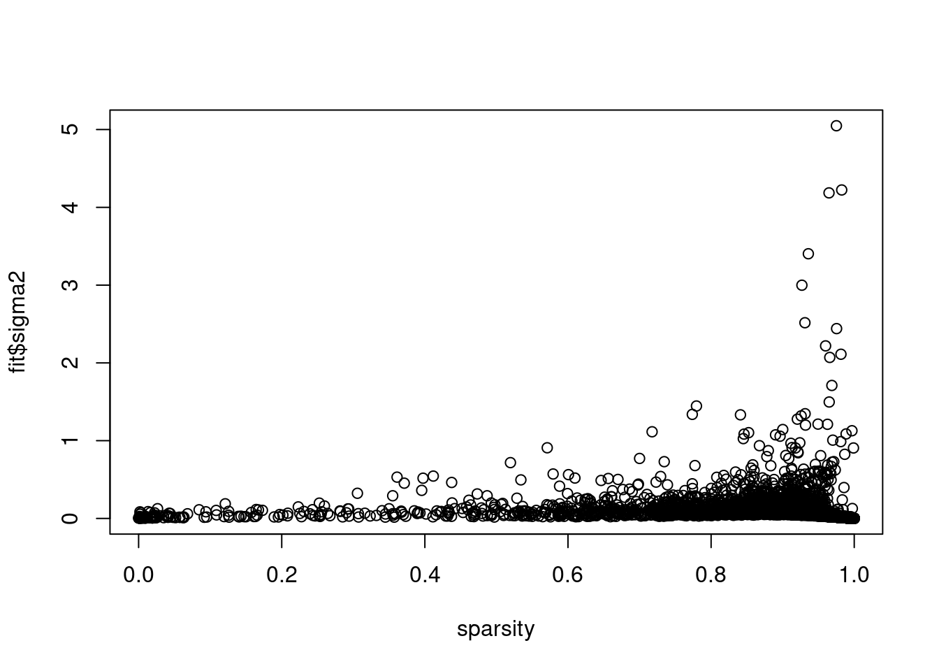
| Version | Author | Date |
|---|---|---|
| 42f0de4 | DongyueXie | 2023-01-05 |
Visualize loadings
source('code/poisson_STM/plot_factors.R')cell_names = as.character(pbmc_facs$samples$subpop)
plot.factors(fit$fit_flash,cell_names,title='splitting PMF')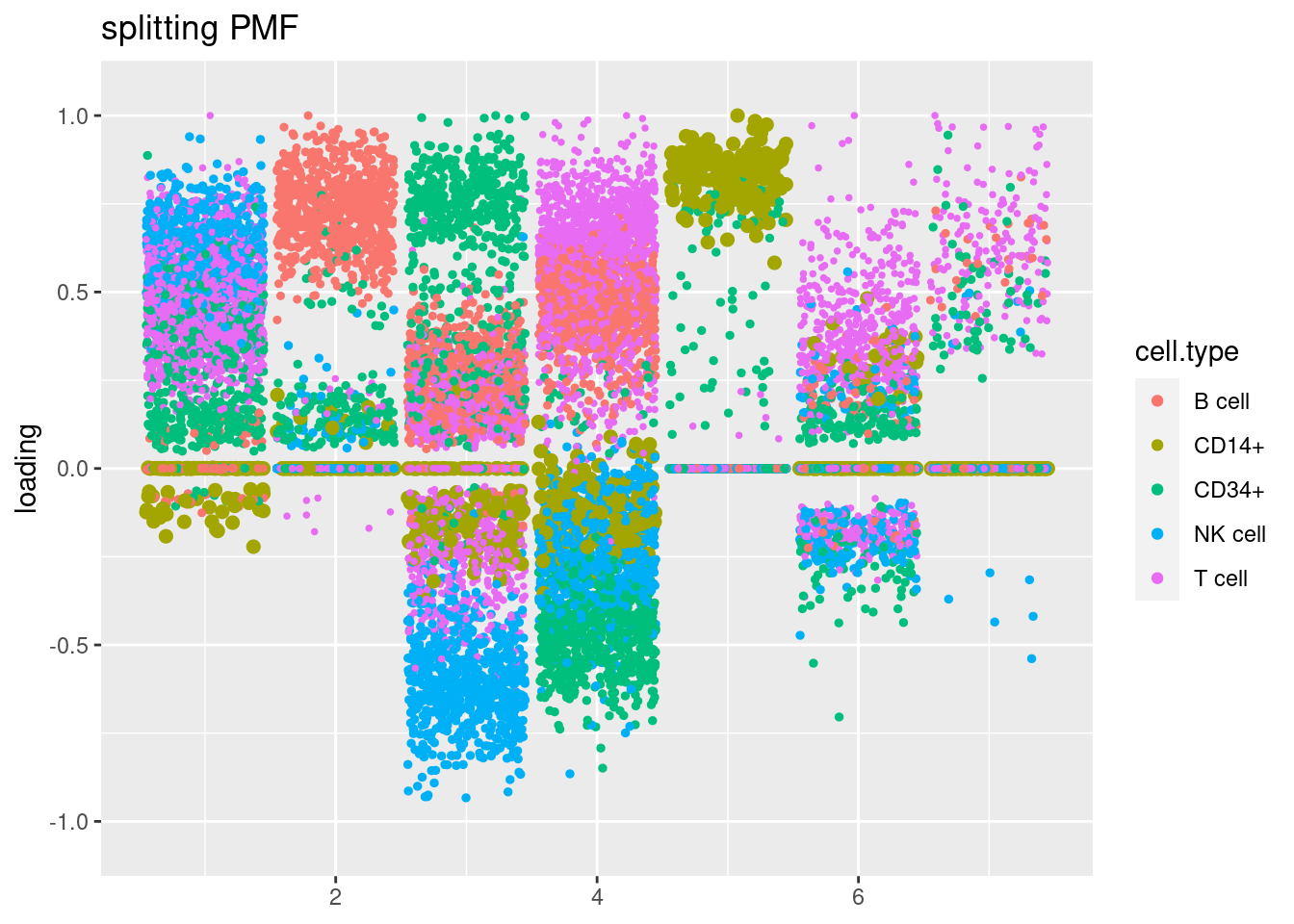
| Version | Author | Date |
|---|---|---|
| 42f0de4 | DongyueXie | 2023-01-05 |
fit_flashier = readRDS('/project2/mstephens/dongyue/poisson_mf/pbmc3k/flash_pbmc3k.rds')
plot.factors(fit_flashier,cell_names,title='flashier')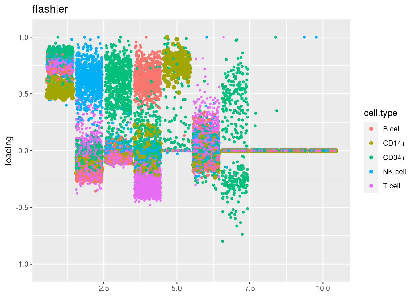
| Version | Author | Date |
|---|---|---|
| 42f0de4 | DongyueXie | 2023-01-05 |
source('code/poisson_STM/plot_factors_general.R')
fit_glmpca_poi = readRDS('/project2/mstephens/dongyue/poisson_mf/pbmc3k/glmpca_pbmc3k_poi.rds')
plot.factors.general(fit_glmpca_poi$loadings,cell_names,title='glmpca poi')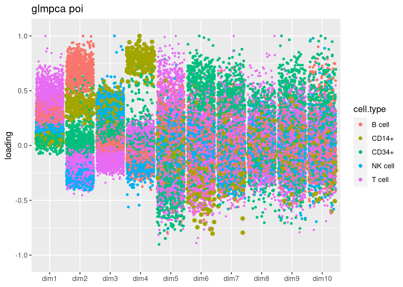
| Version | Author | Date |
|---|---|---|
| 42f0de4 | DongyueXie | 2023-01-05 |
fit_glmpca_nb = readRDS('/project2/mstephens/dongyue/poisson_mf/pbmc3k/glmpca_pbmc3k_nb.rds')
plot.factors.general(fit_glmpca_nb$loadings,cell_names,title='glmpca nb')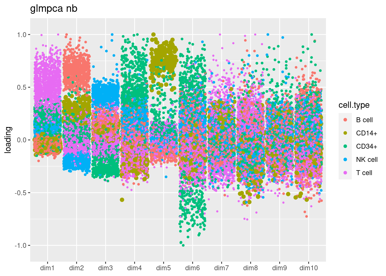
| Version | Author | Date |
|---|---|---|
| 42f0de4 | DongyueXie | 2023-01-05 |
run time analysis
fit$run_timeTime difference of 10.15867 hourslapply(fit$run_time_break_down,mean)$run_time_vga_init
Time difference of 28.89131 secs
$run_time_flash_init
Time difference of 71.49468 secs
$run_time_vga
[1] 11.04436
$run_time_flash_init_factor
[1] 4.846896
$run_time_flash_greedy
[1] 0.4588499
$run_time_flash_backfitting
[1] 13.73861
$run_time_flash_nullcheck
[1] 1.401617Latent variable
Take a look at the latent M in splitting PMF model. M is the posterior mean of \(q_\mu = N(\mu;m,v)\).
What are M’s corresponds to zero Ys? Large Ys?
How does the M compared to GLMPCA’s latent representation?
Histogram of latent variable corresponding to y = 0.
hist(fit$fit_flash$flash.fit$Y[as.vector(counts==0)],breaks=100,xlab='splitting PMF latent var size for those Y=0',main='')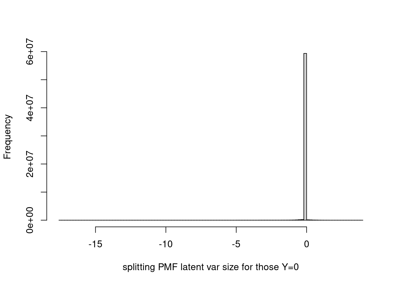
summary(fit$fit_flash$flash.fit$Y[as.vector(counts==0)]) Min. 1st Qu. Median Mean 3rd Qu. Max.
-17.532822 -0.000597 -0.000043 -0.021565 -0.000001 3.997050 It seems that most of them are very close to 0? Let’s set probability = TRUE and restrict ylim to (0,0.2).
hist(fit$fit_flash$flash.fit$Y[as.vector(counts==0)],breaks=200,xlab='splitting PMF latent var size for those Y=0',main='',probability = T,ylim=c(0,0.2))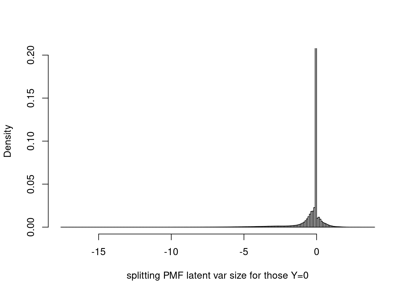
Look at GLMPCA:
hist(tcrossprod(as.matrix(fit_glmpca_poi$loadings),as.matrix(fit_glmpca_poi$factors))[as.vector(counts==0)],breaks=100,xlab='GLMPCA latent var size for those Y=0',main='')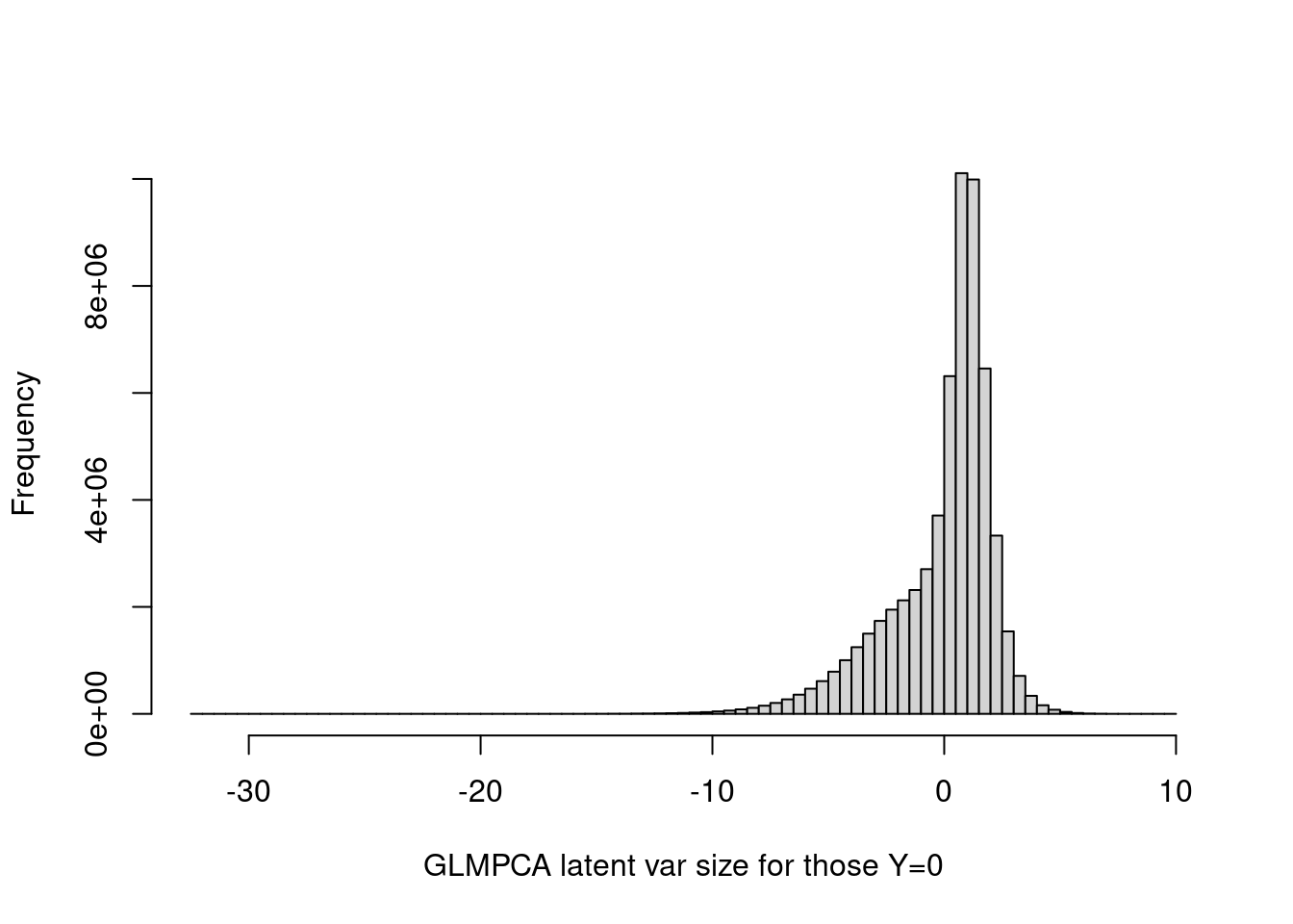
summary(tcrossprod(as.matrix(fit_glmpca_poi$loadings),as.matrix(fit_glmpca_poi$factors))[as.vector(counts==0)]) Min. 1st Qu. Median Mean 3rd Qu. Max.
-32.12124 -0.99826 0.63654 -0.05514 1.36053 9.60655 The GLMPCA latent vraibles are less concentrated around 0. Maybe this is because it does not induce sparsity on L and F.
Histogram of latent variable corresponding to y > 0.
hist(fit$fit_flash$flash.fit$Y[as.vector(counts>0)],breaks=100,xlab='splitting PMF latent var size for those Y>0',main='')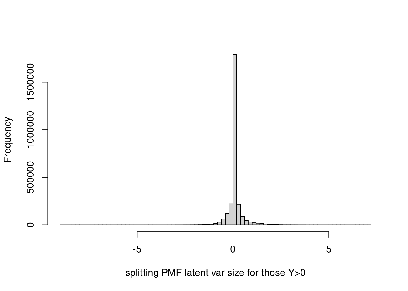
summary(fit$fit_flash$flash.fit$Y[as.vector(counts>0)]) Min. 1st Qu. Median Mean 3rd Qu. Max.
-8.96516 0.01205 0.04553 0.08838 0.11864 7.19377 Let’s limit ylim to (0,1), and set probability = TRUE.
hist(fit$fit_flash$flash.fit$Y[as.vector(counts>0)],breaks=200,xlab='splitting PMF latent var size for those Y>0',main='',ylim=c(0,1),probability = T,col=rgb(1,0,0,1/4))
abline(v = 0,lty=2)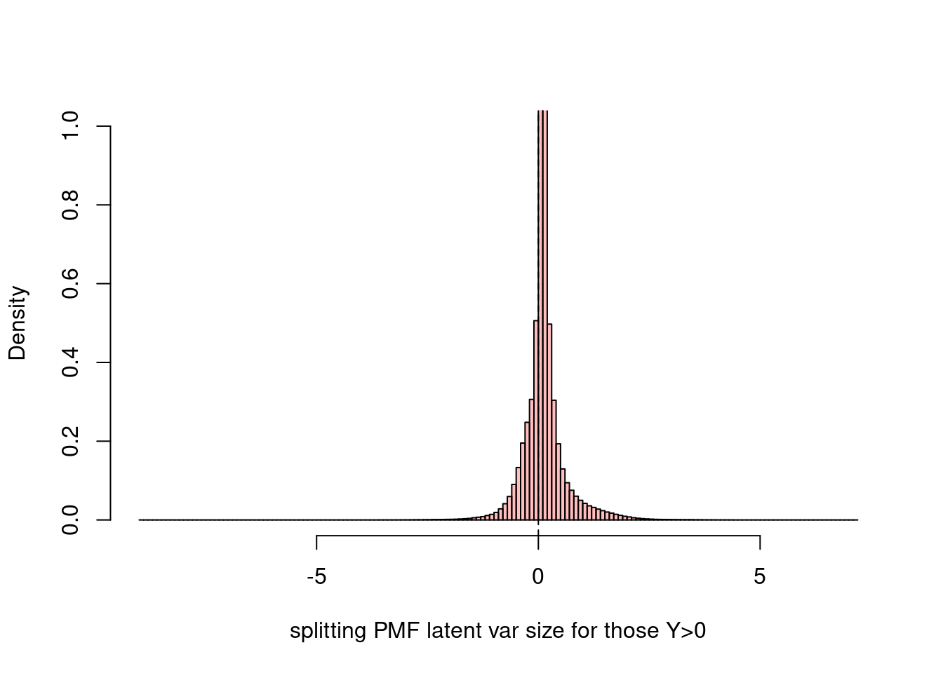
hist(tcrossprod(as.matrix(fit_glmpca_poi$loadings),as.matrix(fit_glmpca_poi$factors))[as.vector(counts>0)],breaks=100,xlab='GLMPCA latent var size for those Y>0',main='')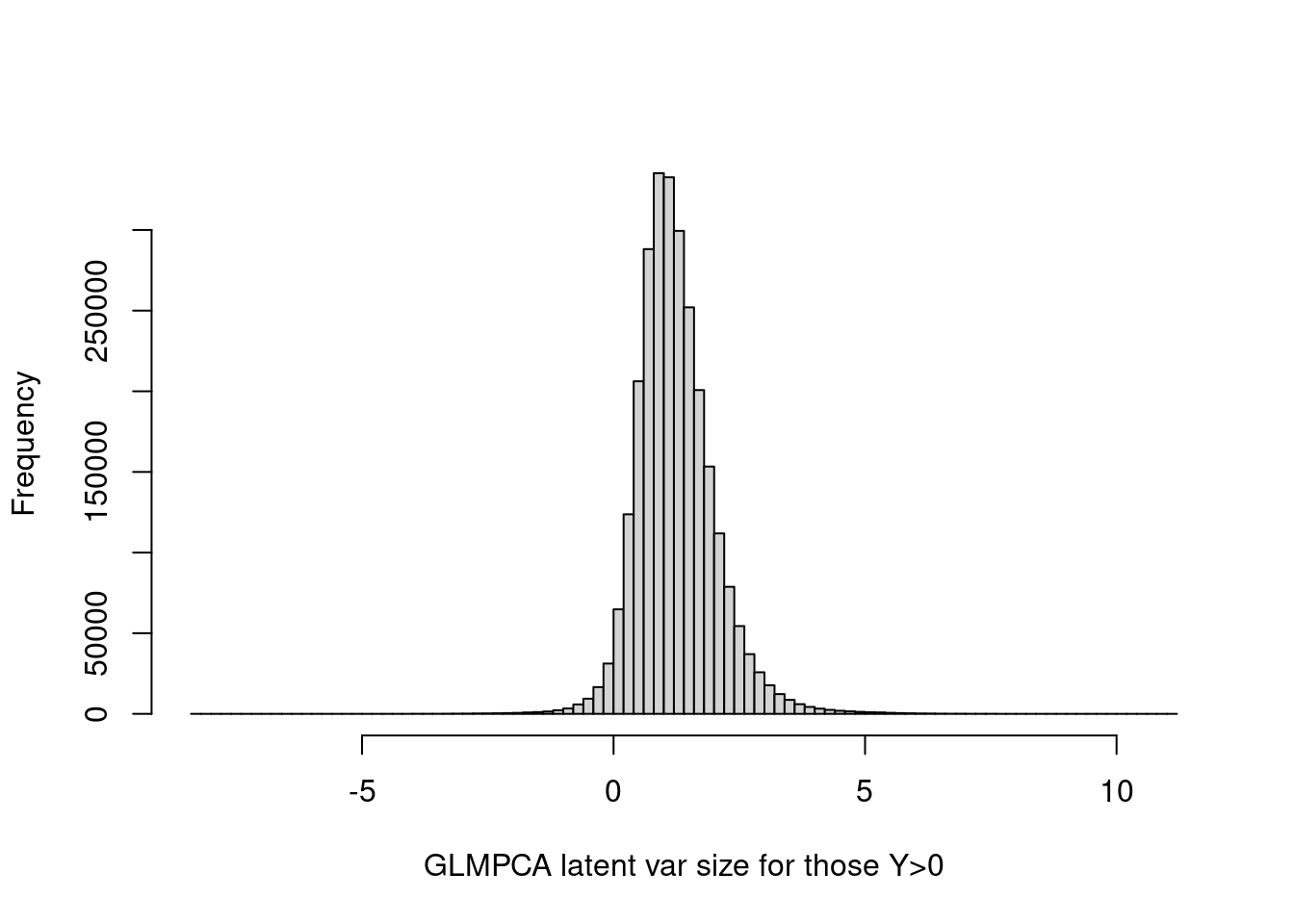
summary(tcrossprod(as.matrix(fit_glmpca_poi$loadings),as.matrix(fit_glmpca_poi$factors))[as.vector(counts>0)]) Min. 1st Qu. Median Mean 3rd Qu. Max.
-8.2505 0.7475 1.1542 1.2377 1.6455 11.1552 Look at how many non-zeros are there in the Y:
hist(log(counts[counts>0]),breaks = 100)<sparse>[ <logic> ]: .M.sub.i.logical() maybe inefficient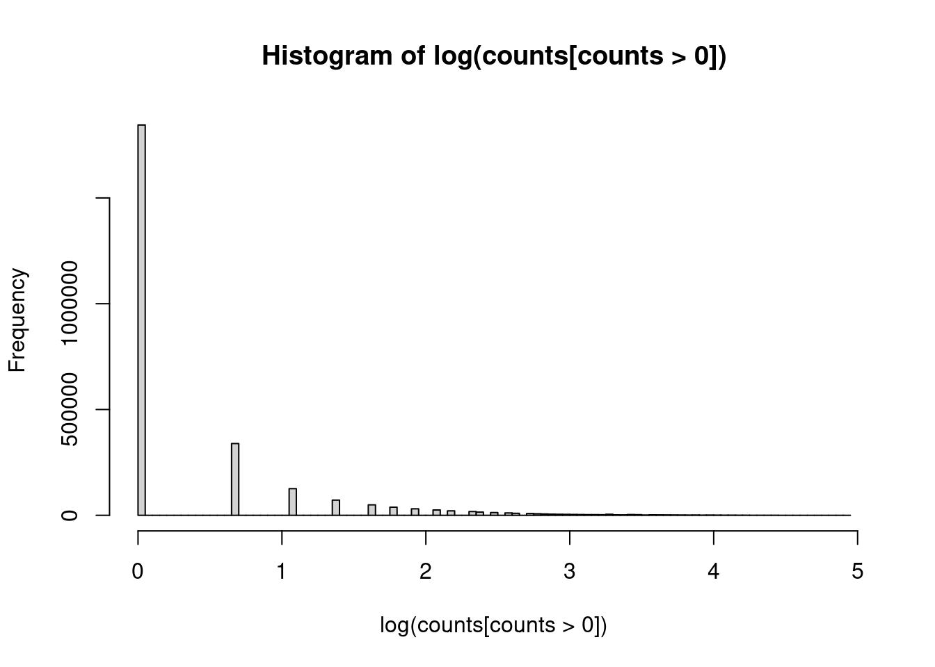
# The latent variable from splitting PMF seems to be very symmetric for those corresponding to $Y>0$.
h_smaller = hist(log(counts[(fit$fit_flash$flash.fit$Y[as.vector(counts>0)])<0]),breaks = 100,main='',xlab='')
h_larger = hist(log(counts[(fit$fit_flash$flash.fit$Y[as.vector(counts>0)])>0]),breaks = 100,main='',xlab='')

plot( h_larger, col=rgb(0,0,1,1/4), xlim=c(0,5))
plot( h_smaller, col=rgb(1,0,0,1/4), xlim=c(0,5),add=T)
legend('topright',c('>0','<0'),fill=c(rgb(0,0,1,1/4),rgb(1,0,0,1/4)),)
sessionInfo()R version 4.1.0 (2021-05-18)
Platform: x86_64-pc-linux-gnu (64-bit)
Running under: CentOS Linux 7 (Core)
Matrix products: default
BLAS: /software/R-4.1.0-no-openblas-el7-x86_64/lib64/R/lib/libRblas.so
LAPACK: /software/R-4.1.0-no-openblas-el7-x86_64/lib64/R/lib/libRlapack.so
locale:
[1] LC_CTYPE=en_US.UTF-8 LC_NUMERIC=C LC_TIME=C
[4] LC_COLLATE=C LC_MONETARY=C LC_MESSAGES=C
[7] LC_PAPER=C LC_NAME=C LC_ADDRESS=C
[10] LC_TELEPHONE=C LC_MEASUREMENT=C LC_IDENTIFICATION=C
attached base packages:
[1] stats graphics grDevices utils datasets methods base
other attached packages:
[1] ggplot2_3.4.0 stm_1.2.8 Matrix_1.5-3 fastTopics_0.6-142
[5] workflowr_1.6.2
loaded via a namespace (and not attached):
[1] mcmc_0.9-7 bitops_1.0-7 matrixStats_0.59.0
[4] fs_1.5.0 progress_1.2.2 httr_1.4.4
[7] rprojroot_2.0.2 tools_4.1.0 bslib_0.2.5.1
[10] utf8_1.2.2 R6_2.5.1 irlba_2.3.5.1
[13] uwot_0.1.14 DBI_1.1.1 lazyeval_0.2.2
[16] colorspace_2.0-3 withr_2.5.0 wavethresh_4.7.2
[19] tidyselect_1.2.0 prettyunits_1.1.1 ebpm_0.0.1.3
[22] compiler_4.1.0 git2r_0.28.0 cli_3.5.0
[25] quantreg_5.94 SparseM_1.81 plotly_4.10.1
[28] labeling_0.4.2 horseshoe_0.2.0 sass_0.4.0
[31] smashrgen_1.1.1 caTools_1.18.2 flashier_0.2.34
[34] scales_1.2.1 SQUAREM_2021.1 quadprog_1.5-8
[37] pbapply_1.6-0 mixsqp_0.3-48 stringr_1.4.0
[40] digest_0.6.30 rmarkdown_2.9 deconvolveR_1.2-1
[43] MCMCpack_1.6-3 vebpm_0.3.8 pkgconfig_2.0.3
[46] htmltools_0.5.3 highr_0.9 fastmap_1.1.0
[49] invgamma_1.1 htmlwidgets_1.5.4 rlang_1.0.6
[52] rstudioapi_0.13 farver_2.1.1 jquerylib_0.1.4
[55] generics_0.1.3 jsonlite_1.8.3 dplyr_1.0.10
[58] magrittr_2.0.3 smashr_1.3-6 Rcpp_1.0.9
[61] munsell_0.5.0 fansi_1.0.3 RcppZiggurat_0.1.6
[64] lifecycle_1.0.3 stringi_1.6.2 whisker_0.4
[67] yaml_2.3.6 MASS_7.3-54 plyr_1.8.6
[70] Rtsne_0.16 grid_4.1.0 parallel_4.1.0
[73] promises_1.2.0.1 ggrepel_0.9.2 crayon_1.5.2
[76] lattice_0.20-44 cowplot_1.1.1 splines_4.1.0
[79] hms_1.1.2 knitr_1.33 pillar_1.8.1
[82] softImpute_1.4-1 reshape2_1.4.4 glue_1.6.2
[85] evaluate_0.14 trust_0.1-8 data.table_1.14.6
[88] RcppParallel_5.1.5 nloptr_1.2.2.2 vctrs_0.5.1
[91] httpuv_1.6.1 MatrixModels_0.5-1 gtable_0.3.1
[94] purrr_0.3.5 ebnm_1.0-11 tidyr_1.2.1
[97] assertthat_0.2.1 ashr_2.2-54 xfun_0.24
[100] Rfast_2.0.6 NNLM_0.4.4 coda_0.19-4
[103] later_1.3.0 survival_3.2-11 viridisLite_0.4.1
[106] glmpca_0.2.0 truncnorm_1.0-8 tibble_3.1.8
[109] ellipsis_0.3.2