splitting PMF 1 backfitting in init
DongyueXie
2022-12-13
Last updated: 2022-12-17
Checks: 7 0
Knit directory: gsmash/
This reproducible R Markdown analysis was created with workflowr (version 1.6.2). The Checks tab describes the reproducibility checks that were applied when the results were created. The Past versions tab lists the development history.
Great! Since the R Markdown file has been committed to the Git repository, you know the exact version of the code that produced these results.
Great job! The global environment was empty. Objects defined in the global environment can affect the analysis in your R Markdown file in unknown ways. For reproduciblity it’s best to always run the code in an empty environment.
The command set.seed(20220606) was run prior to running
the code in the R Markdown file. Setting a seed ensures that any results
that rely on randomness, e.g. subsampling or permutations, are
reproducible.
Great job! Recording the operating system, R version, and package versions is critical for reproducibility.
Nice! There were no cached chunks for this analysis, so you can be confident that you successfully produced the results during this run.
Great job! Using relative paths to the files within your workflowr project makes it easier to run your code on other machines.
Great! You are using Git for version control. Tracking code development and connecting the code version to the results is critical for reproducibility.
The results in this page were generated with repository version 84b3d02. See the Past versions tab to see a history of the changes made to the R Markdown and HTML files.
Note that you need to be careful to ensure that all relevant files for
the analysis have been committed to Git prior to generating the results
(you can use wflow_publish or
wflow_git_commit). workflowr only checks the R Markdown
file, but you know if there are other scripts or data files that it
depends on. Below is the status of the Git repository when the results
were generated:
Ignored files:
    Ignored:    .Rhistory
    Ignored:    .Rproj.user/

Unstaged changes:
    Modified:   analysis/index.Rmd
Note that any generated files, e.g. HTML, png, CSS, etc., are not included in this status report because it is ok for generated content to have uncommitted changes.
These are the previous versions of the repository in which changes were
made to the R Markdown
(analysis/splitting_PMF_1backfitinit.Rmd) and HTML
(docs/splitting_PMF_1backfitinit.html) files. If you’ve
configured a remote Git repository (see ?wflow_git_remote),
click on the hyperlinks in the table below to view the files as they
were in that past version.
| File | Version | Author | Date | Message |
|---|---|---|---|---|
| Rmd | 84b3d02 | DongyueXie | 2022-12-17 | wflow_publish("analysis/splitting_PMF_1backfitinit.Rmd") |
Introduction
The results here show that using 1 back-fitting in flash initialization does not affect the final results.
rmse = function(x,y){return(sqrt(mean((x-y)^2)))}
res = readRDS('/project2/mstephens/dongyue/poisson_mf/PMF10_K3simu_pbmc_3cells_1backinit.rds')
We first look at the number factors recovered from both methods. The true \(K\) is 3.
K_hat = c()
for(i in 1:length(res$output)){
  K_hat = rbind(K_hat,c(res$output[[i]]$fitted_model$flash$n.factors,res$output[[i]]$fitted_model$splitting$fit_flash$n.factors))
}
colnames(K_hat) = c('flash','splittingPMF')
K_hat
flash splittingPMF
[1,] 8 3
[2,] 12 3
[3,] 6 3
[4,] 7 3
[5,] 6 3
[6,] 8 3
[7,] 8 3
[8,] 10 3
[9,] 13 3
[10,] 5 3Next we compare \(\hat L\hat F'\) and true \(LF'\).
fit = readRDS('/project2/mstephens/dongyue/poisson_mf/pbmc_3cells_Sij.rds')
kset = order(fit$fit$fit_flash$pve,decreasing = TRUE)[1:3]
Ltrue = fit$fit$fit_flash$L.pm[,kset]
Ftrue = fit$fit$fit_flash$F.pm[,kset]
Mu_true = tcrossprod(Ltrue,Ftrue)
rmses= c()
for(i in 1:length(res$output)){
rmses = rbind(rmses,c(rmse(Mu_true,fitted(res$output[[i]]$fitted_model$flash)),rmse(Mu_true,fitted(res$output[[i]]$fitted_model$splitting$fit_flash))))
}
colnames(rmses) = c('flash','splittingPMF')
rmses flash splittingPMF
[1,] 0.5819739 0.1742745
[2,] 0.5819058 0.1763028
[3,] 0.5815135 0.1732575
[4,] 0.5817050 0.1724475
[5,] 0.5823862 0.1709836
[6,] 0.5809864 0.1773127
[7,] 0.5816003 0.1786152
[8,] 0.5814658 0.1785925
[9,] 0.5821286 0.1762915
[10,] 0.5815670 0.1660298par(mfrow=c(2,1))
for(i in 1:length(res$output)){
plot(fitted(res$output[[i]]$fitted_model$flash),Mu_true,col='grey80',xlab='fitted',ylab='LF',main='flash')
abline(a=0,b=1)
plot(fitted(res$output[[i]]$fitted_model$splitting$fit_flash),Mu_true,col='grey80',xlab='fitted',ylab='LF',main='splitting')
abline(a=0,b=1)
}
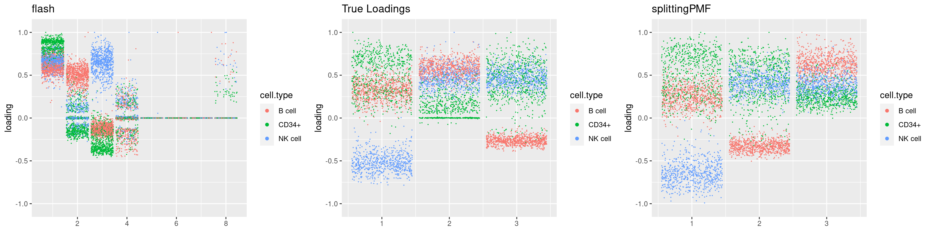
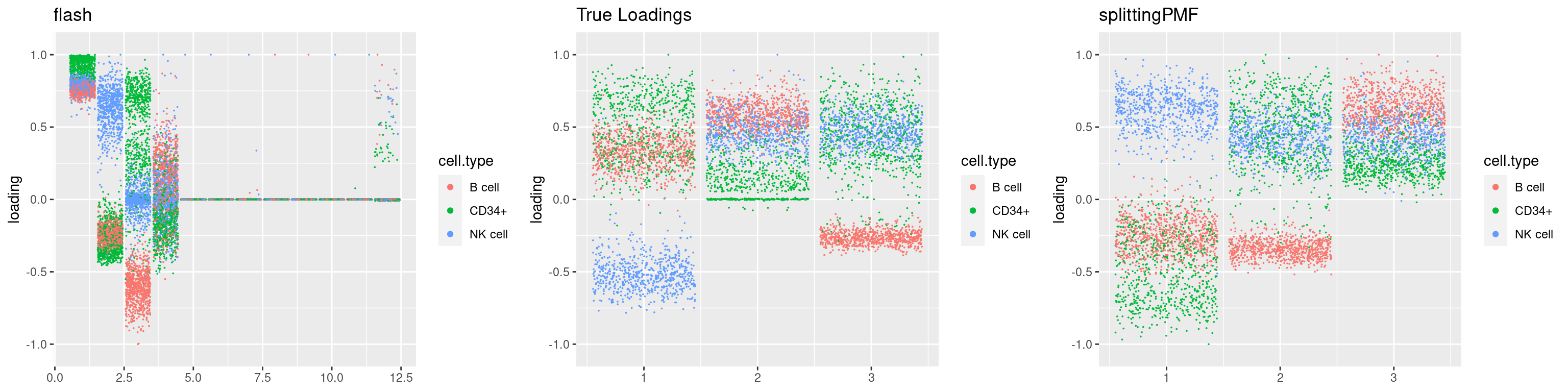
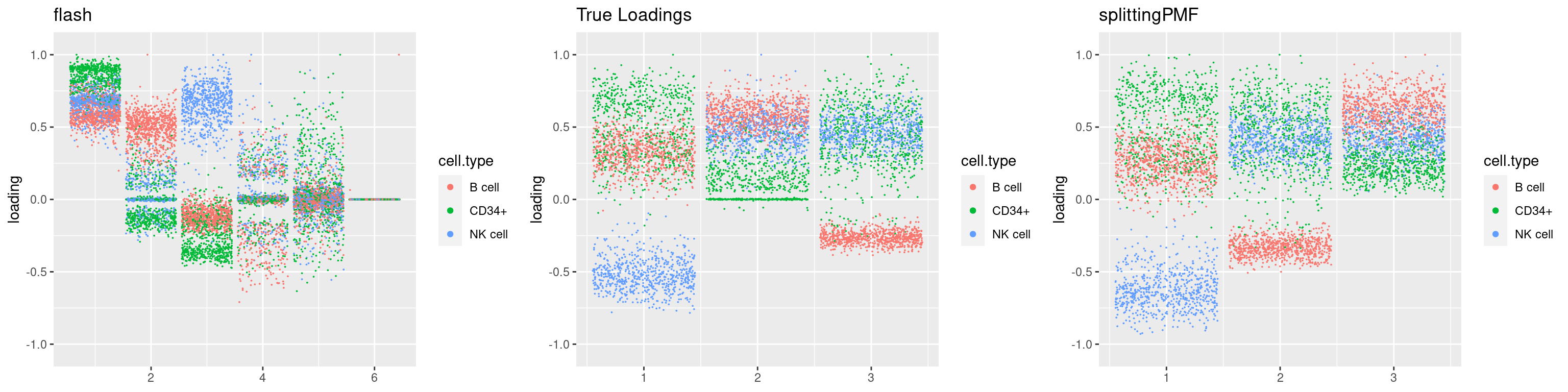
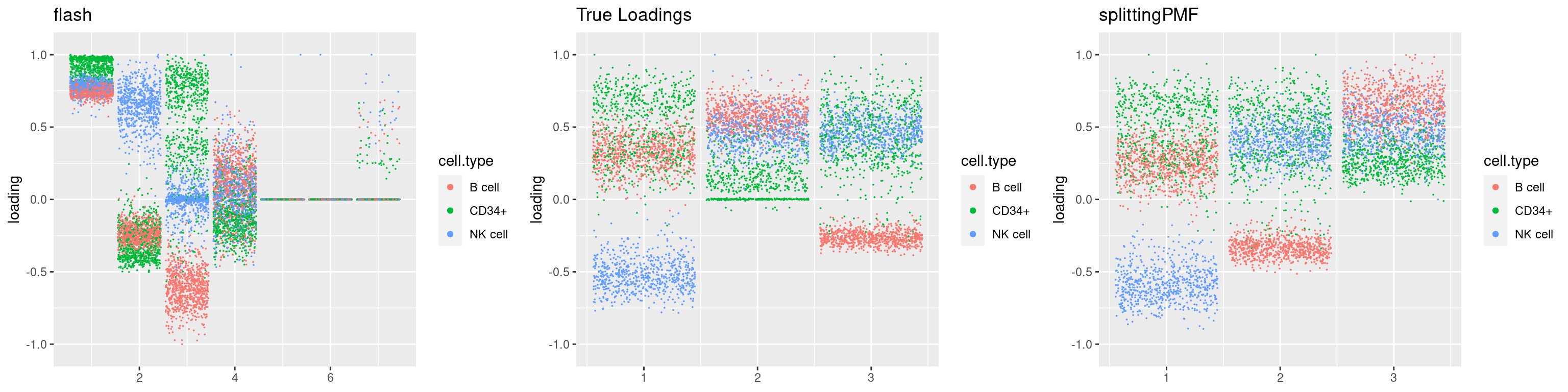
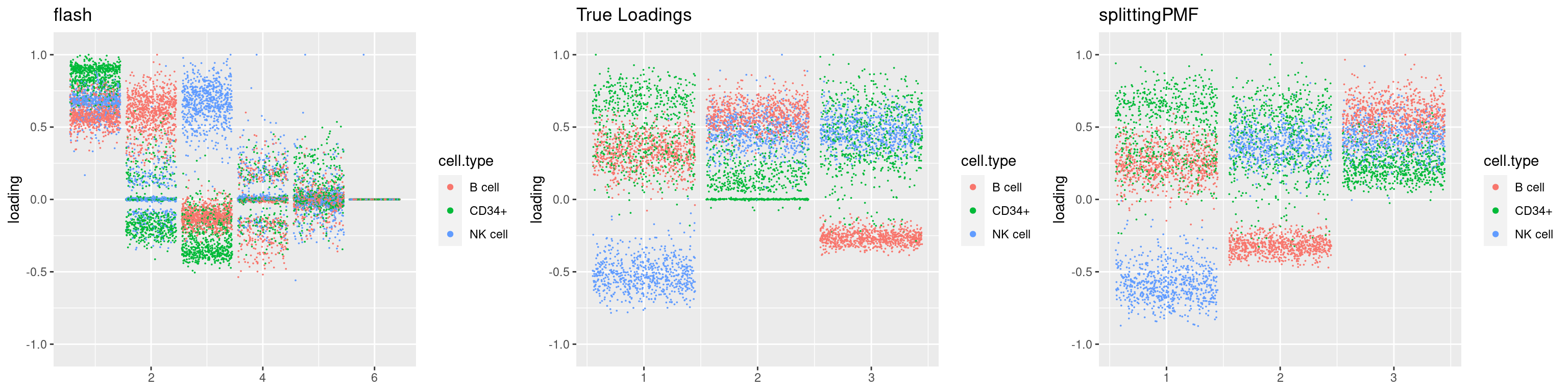
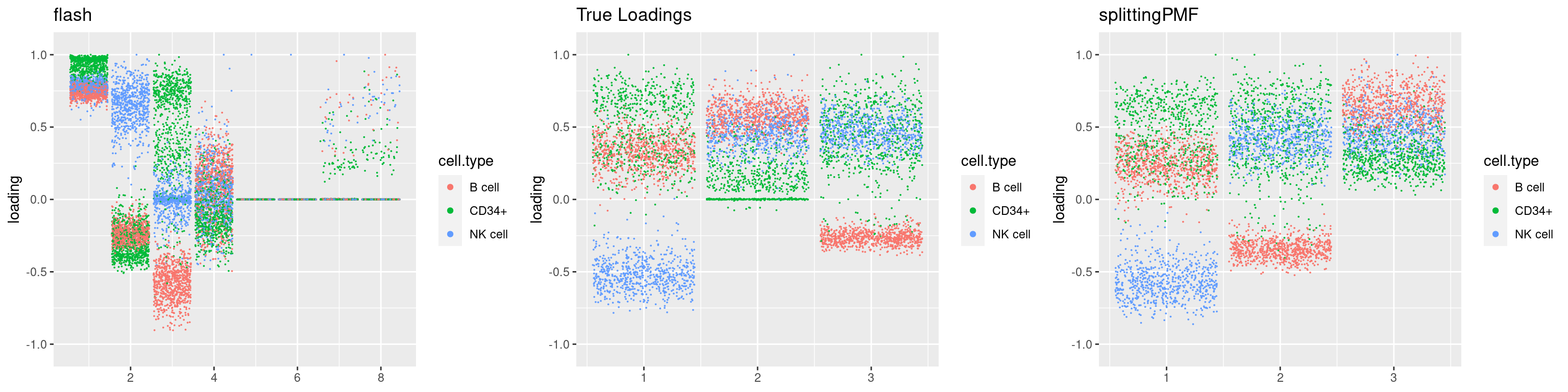
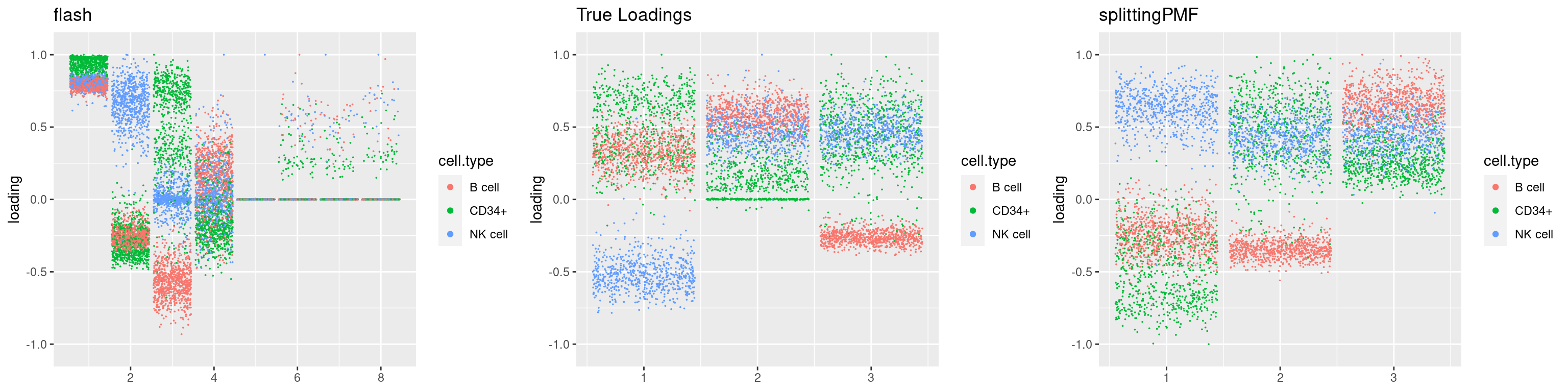
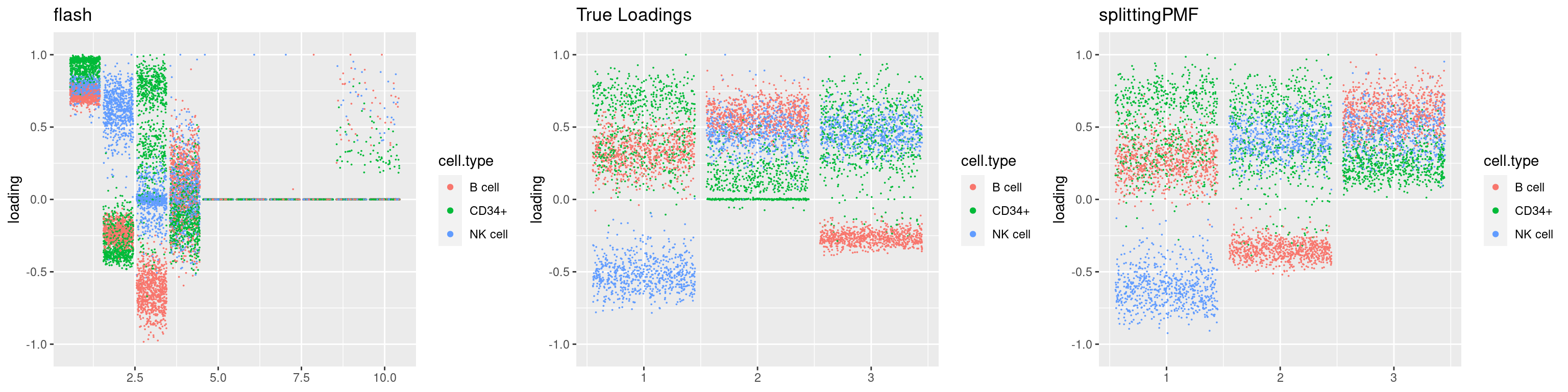
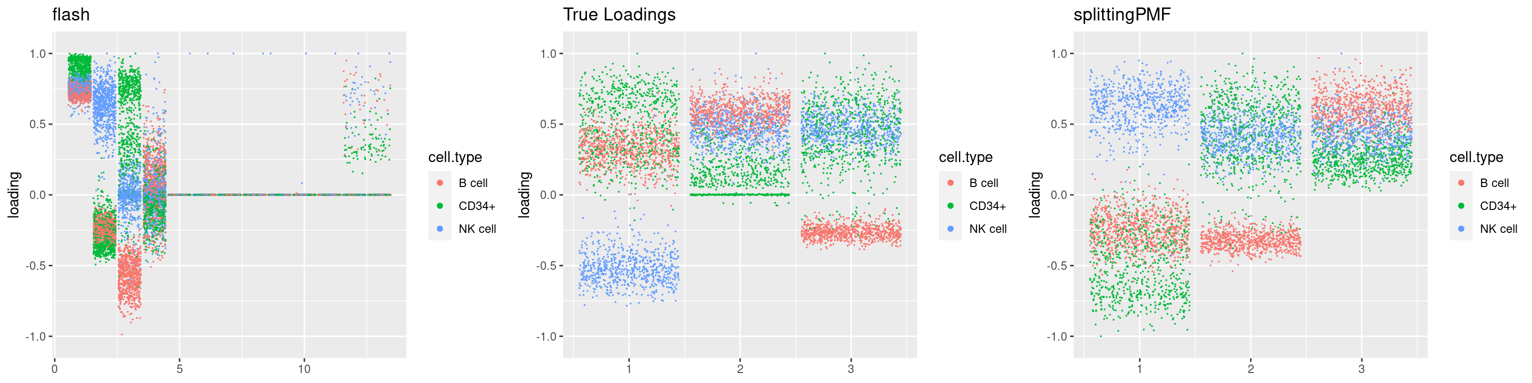
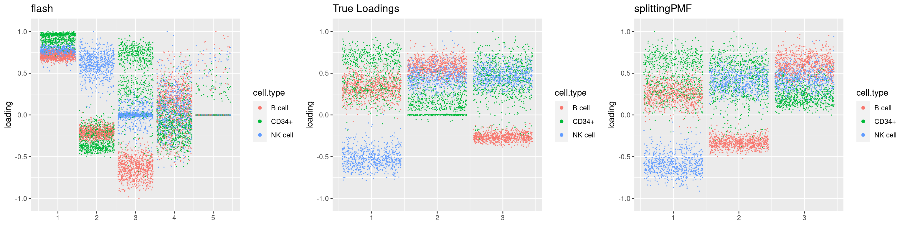
par(mfrow=c(1,1))Next we look at how the structures of L and F are recovered by both methods.
We first plot loadings.
library(fastTopics)
library(Matrix)
library(stm)
require(gridExtra)
Loading required package: gridExtradata(pbmc_facs)
counts <- pbmc_facs$counts
table(pbmc_facs$samples$subpop)
 B cell   CD14+   CD34+ NK cell  T cell
    767     163     687     673    1484
## use only B cell and NK cell and CD34+
cells = pbmc_facs$samples$subpop%in%c('B cell', 'NK cell','CD34+')
counts = counts[cells,]
# filter out genes that has few expressions(3% cells)
genes = (colSums(counts>0) > 0.03*dim(counts)[1])
cell_names = pbmc_facs$samples$subpop[cells]
source('code/poisson_STM/plot_factors.R')plot0=plot.factors(fit$fit$fit_flash,cell.types=cell_names,kset=kset,title='True Loadings')
for(i in 1:length(res$output)){
plot1 = plot.factors(res$output[[i]]$fitted_model$flash,cell.types=cell_names,title='flash')
plot2 = plot.factors(res$output[[i]]$fitted_model$splitting$fit_flash,cell.types=cell_names,title='splittingPMF')
grid.arrange(plot1, plot0,plot2, ncol=3)
}
misc
number of iterations until convergence
for(i in 1:length(res$output)){
   print(length(res$output[[i]]$fitted_model$splitting$eblo_trace))
}
[1] 88
[1] 90
[1] 92
[1] 90
[1] 88
[1] 87
[1] 88
[1] 85
[1] 86
[1] 90run time analysis
for(i in 1:length(res$output)){
   print((res$output[[i]]$fitted_model$splitting$run_time))
}
Time difference of 15.33213 mins
Time difference of 16.28081 mins
Time difference of 16.98529 mins
Time difference of 16.27841 mins
Time difference of 16.96993 mins
Time difference of 14.47638 mins
Time difference of 16.00253 mins
Time difference of 15.43373 mins
Time difference of 15.69402 mins
Time difference of 16.36275 minsrun time break down
tt = c()
for(i in 1:length(res$output)){
   tt = rbind(tt,unlist(lapply(res$output[[i]]$fitted_model$splitting$run_time_break_down,mean)))
}
apply(tt,2,mean)
run_time_vga_init run_time_vga
187.4276577 4.0366805
run_time_flash_init run_time_flash_init_factor
0.2409684 0.3362548
run_time_flash_greedy run_time_flash_backfitting
1.5484761 1.4630587
run_time_flash_nullcheck
0.1801452 Plot K trace
plot(res$output[[i]]$fitted_model$splitting$K_trace,ylab='K',xlab='iterations',type='l',col='grey80')
for(i in 1:length(res$output)){
   lines(res$output[[i]]$fitted_model$splitting$K_trace,col=i)
}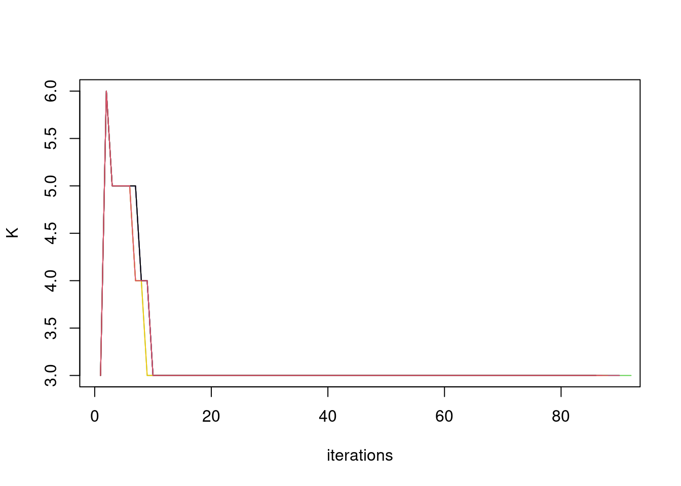
Maybe omit greedy step after the K is stabilized? to reduce computation time.
sessionInfo()R version 4.1.0 (2021-05-18)
Platform: x86_64-pc-linux-gnu (64-bit)
Running under: CentOS Linux 7 (Core)
Matrix products: default
BLAS: /software/R-4.1.0-no-openblas-el7-x86_64/lib64/R/lib/libRblas.so
LAPACK: /software/R-4.1.0-no-openblas-el7-x86_64/lib64/R/lib/libRlapack.so
locale:
[1] LC_CTYPE=en_US.UTF-8 LC_NUMERIC=C LC_TIME=C
[4] LC_COLLATE=C LC_MONETARY=C LC_MESSAGES=C
[7] LC_PAPER=C LC_NAME=C LC_ADDRESS=C
[10] LC_TELEPHONE=C LC_MEASUREMENT=C LC_IDENTIFICATION=C
attached base packages:
[1] stats graphics grDevices utils datasets methods base
other attached packages:
[1] ggplot2_3.4.0 gridExtra_2.3 stm_1.1.6 Matrix_1.5-3
[5] fastTopics_0.6-142 workflowr_1.6.2
loaded via a namespace (and not attached):
[1] mcmc_0.9-7 bitops_1.0-7 matrixStats_0.59.0
[4] fs_1.5.0 progress_1.2.2 httr_1.4.4
[7] rprojroot_2.0.2 tools_4.1.0 bslib_0.2.5.1
[10] utf8_1.2.2 R6_2.5.1 irlba_2.3.5.1
[13] uwot_0.1.14 DBI_1.1.1 lazyeval_0.2.2
[16] colorspace_2.0-3 withr_2.5.0 wavethresh_4.7.2
[19] tidyselect_1.2.0 prettyunits_1.1.1 ebpm_0.0.1.3
[22] compiler_4.1.0 git2r_0.28.0 cli_3.4.1
[25] quantreg_5.94 SparseM_1.81 plotly_4.10.1
[28] labeling_0.4.2 horseshoe_0.2.0 sass_0.4.0
[31] caTools_1.18.2 flashier_0.2.34 scales_1.2.1
[34] SQUAREM_2021.1 quadprog_1.5-8 pbapply_1.6-0
[37] mixsqp_0.3-48 stringr_1.4.0 digest_0.6.30
[40] rmarkdown_2.9 MCMCpack_1.6-3 deconvolveR_1.2-1
[43] vebpm_0.3.3 pkgconfig_2.0.3 htmltools_0.5.3
[46] highr_0.9 fastmap_1.1.0 invgamma_1.1
[49] htmlwidgets_1.5.4 rlang_1.0.6 rstudioapi_0.13
[52] farver_2.1.1 jquerylib_0.1.4 generics_0.1.3
[55] jsonlite_1.8.3 dplyr_1.0.10 magrittr_2.0.3
[58] smashr_1.3-6 Rcpp_1.0.9 munsell_0.5.0
[61] fansi_1.0.3 lifecycle_1.0.3 stringi_1.6.2
[64] whisker_0.4 yaml_2.3.6 nleqslv_3.3.3
[67] rootSolve_1.8.2.3 MASS_7.3-54 plyr_1.8.6
[70] Rtsne_0.16 grid_4.1.0 parallel_4.1.0
[73] promises_1.2.0.1 ggrepel_0.9.2 crayon_1.5.2
[76] lattice_0.20-44 cowplot_1.1.1 splines_4.1.0
[79] hms_1.1.2 knitr_1.33 pillar_1.8.1
[82] softImpute_1.4-1 reshape2_1.4.4 glue_1.6.2
[85] evaluate_0.14 trust_0.1-8 data.table_1.14.6
[88] RcppParallel_5.1.5 nloptr_1.2.2.2 vctrs_0.5.1
[91] httpuv_1.6.1 MatrixModels_0.5-1 gtable_0.3.1
[94] purrr_0.3.5 ebnm_1.0-11 tidyr_1.2.1
[97] assertthat_0.2.1 ashr_2.2-54 xfun_0.24
[100] NNLM_0.4.4 coda_0.19-4 later_1.3.0
[103] survival_3.2-11 viridisLite_0.4.1 truncnorm_1.0-8
[106] tibble_3.1.8 ellipsis_0.3.2