blasso_bimodal_example
Matthew Stephens
2020-06-04
Last updated: 2020-06-04
Checks: 7 0
Knit directory: misc/analysis/
This reproducible R Markdown analysis was created with workflowr (version 1.6.1). The Checks tab describes the reproducibility checks that were applied when the results were created. The Past versions tab lists the development history.
Great! Since the R Markdown file has been committed to the Git repository, you know the exact version of the code that produced these results.
Great job! The global environment was empty. Objects defined in the global environment can affect the analysis in your R Markdown file in unknown ways. For reproduciblity it’s best to always run the code in an empty environment.
The command set.seed(1) was run prior to running the code in the R Markdown file. Setting a seed ensures that any results that rely on randomness, e.g. subsampling or permutations, are reproducible.
Great job! Recording the operating system, R version, and package versions is critical for reproducibility.
Nice! There were no cached chunks for this analysis, so you can be confident that you successfully produced the results during this run.
Great job! Using relative paths to the files within your workflowr project makes it easier to run your code on other machines.
Great! You are using Git for version control. Tracking code development and connecting the code version to the results is critical for reproducibility.
The results in this page were generated with repository version 6513b8e. See the Past versions tab to see a history of the changes made to the R Markdown and HTML files.
Note that you need to be careful to ensure that all relevant files for the analysis have been committed to Git prior to generating the results (you can use wflow_publish or wflow_git_commit). workflowr only checks the R Markdown file, but you know if there are other scripts or data files that it depends on. Below is the status of the Git repository when the results were generated:
Ignored files:
    Ignored:    .DS_Store
    Ignored:    .Rhistory
    Ignored:    .Rproj.user/
    Ignored:    analysis/.RData
    Ignored:    analysis/.Rhistory
    Ignored:    analysis/ALStruct_cache/
    Ignored:    data/.Rhistory
    Ignored:    data/pbmc/

Untracked files:
    Untracked:  .dropbox
    Untracked:  Icon
    Untracked:  analysis/GHstan.Rmd
    Untracked:  analysis/GTEX-cogaps.Rmd
    Untracked:  analysis/PACS.Rmd
    Untracked:  analysis/Rplot.png
    Untracked:  analysis/SPCAvRP.rmd
    Untracked:  analysis/admm_02.Rmd
    Untracked:  analysis/admm_03.Rmd
    Untracked:  analysis/compare-transformed-models.Rmd
    Untracked:  analysis/cormotif.Rmd
    Untracked:  analysis/cp_ash.Rmd
    Untracked:  analysis/eQTL.perm.rand.pdf
    Untracked:  analysis/eb_prepilot.Rmd
    Untracked:  analysis/eb_var.Rmd
    Untracked:  analysis/ebpmf1.Rmd
    Untracked:  analysis/flash_test_tree.Rmd
    Untracked:  analysis/ieQTL.perm.rand.pdf
    Untracked:  analysis/m6amash.Rmd
    Untracked:  analysis/mash_bhat_z.Rmd
    Untracked:  analysis/mash_ieqtl_permutations.Rmd
    Untracked:  analysis/mixsqp.Rmd
    Untracked:  analysis/mr_ash_modular.Rmd
    Untracked:  analysis/mr_ash_parameterization.Rmd
    Untracked:  analysis/mr_ash_pen.Rmd
    Untracked:  analysis/nejm.Rmd
    Untracked:  analysis/normalize.Rmd
    Untracked:  analysis/pbmc.Rmd
    Untracked:  analysis/poisson_transform.Rmd
    Untracked:  analysis/pseudodata.Rmd
    Untracked:  analysis/qrnotes.txt
    Untracked:  analysis/ridge_iterative_02.Rmd
    Untracked:  analysis/ridge_iterative_splitting.Rmd
    Untracked:  analysis/sc_bimodal.Rmd
    Untracked:  analysis/shrinkage_comparisons_changepoints.Rmd
    Untracked:  analysis/susie_en.Rmd
    Untracked:  analysis/susie_z_investigate.Rmd
    Untracked:  analysis/svd-timing.Rmd
    Untracked:  analysis/temp.RDS
    Untracked:  analysis/temp.Rmd
    Untracked:  analysis/test-figure/
    Untracked:  analysis/test.Rmd
    Untracked:  analysis/test.Rpres
    Untracked:  analysis/test.md
    Untracked:  analysis/test_qr.R
    Untracked:  analysis/test_sparse.Rmd
    Untracked:  analysis/z.txt
    Untracked:  code/multivariate_testfuncs.R
    Untracked:  code/rqb.hacked.R
    Untracked:  data/4matthew/
    Untracked:  data/4matthew2/
    Untracked:  data/E-MTAB-2805.processed.1/
    Untracked:  data/ENSG00000156738.Sim_Y2.RDS
    Untracked:  data/GDS5363_full.soft.gz
    Untracked:  data/GSE41265_allGenesTPM.txt
    Untracked:  data/Muscle_Skeletal.ACTN3.pm1Mb.RDS
    Untracked:  data/Thyroid.FMO2.pm1Mb.RDS
    Untracked:  data/bmass.HaemgenRBC2016.MAF01.Vs2.MergedDataSources.200kRanSubset.ChrBPMAFMarkerZScores.vs1.txt.gz
    Untracked:  data/bmass.HaemgenRBC2016.Vs2.NewSNPs.ZScores.hclust.vs1.txt
    Untracked:  data/bmass.HaemgenRBC2016.Vs2.PreviousSNPs.ZScores.hclust.vs1.txt
    Untracked:  data/eb_prepilot/
    Untracked:  data/finemap_data/fmo2.sim/b.txt
    Untracked:  data/finemap_data/fmo2.sim/dap_out.txt
    Untracked:  data/finemap_data/fmo2.sim/dap_out2.txt
    Untracked:  data/finemap_data/fmo2.sim/dap_out2_snp.txt
    Untracked:  data/finemap_data/fmo2.sim/dap_out_snp.txt
    Untracked:  data/finemap_data/fmo2.sim/data
    Untracked:  data/finemap_data/fmo2.sim/fmo2.sim.config
    Untracked:  data/finemap_data/fmo2.sim/fmo2.sim.k
    Untracked:  data/finemap_data/fmo2.sim/fmo2.sim.k4.config
    Untracked:  data/finemap_data/fmo2.sim/fmo2.sim.k4.snp
    Untracked:  data/finemap_data/fmo2.sim/fmo2.sim.ld
    Untracked:  data/finemap_data/fmo2.sim/fmo2.sim.snp
    Untracked:  data/finemap_data/fmo2.sim/fmo2.sim.z
    Untracked:  data/finemap_data/fmo2.sim/pos.txt
    Untracked:  data/logm.csv
    Untracked:  data/m.cd.RDS
    Untracked:  data/m.cdu.old.RDS
    Untracked:  data/m.new.cd.RDS
    Untracked:  data/m.old.cd.RDS
    Untracked:  data/mainbib.bib.old
    Untracked:  data/mat.csv
    Untracked:  data/mat.txt
    Untracked:  data/mat_new.csv
    Untracked:  data/matrix_lik.rds
    Untracked:  data/paintor_data/
    Untracked:  data/temp.txt
    Untracked:  data/y.txt
    Untracked:  data/y_f.txt
    Untracked:  data/zscore_jointLCLs_m6AQTLs_susie_eQTLpruned.rds
    Untracked:  data/zscore_jointLCLs_random.rds
    Untracked:  explore_udi.R
    Untracked:  output/fit.k10.rds
    Untracked:  output/fit.varbvs.RDS
    Untracked:  output/glmnet.fit.RDS
    Untracked:  output/test.bv.txt
    Untracked:  output/test.gamma.txt
    Untracked:  output/test.hyp.txt
    Untracked:  output/test.log.txt
    Untracked:  output/test.param.txt
    Untracked:  output/test2.bv.txt
    Untracked:  output/test2.gamma.txt
    Untracked:  output/test2.hyp.txt
    Untracked:  output/test2.log.txt
    Untracked:  output/test2.param.txt
    Untracked:  output/test3.bv.txt
    Untracked:  output/test3.gamma.txt
    Untracked:  output/test3.hyp.txt
    Untracked:  output/test3.log.txt
    Untracked:  output/test3.param.txt
    Untracked:  output/test4.bv.txt
    Untracked:  output/test4.gamma.txt
    Untracked:  output/test4.hyp.txt
    Untracked:  output/test4.log.txt
    Untracked:  output/test4.param.txt
    Untracked:  output/test5.bv.txt
    Untracked:  output/test5.gamma.txt
    Untracked:  output/test5.hyp.txt
    Untracked:  output/test5.log.txt
    Untracked:  output/test5.param.txt

Unstaged changes:
    Modified:   analysis/ash_delta_operator.Rmd
    Modified:   analysis/ash_pois_bcell.Rmd
    Modified:   analysis/lasso_em.Rmd
    Modified:   analysis/minque.Rmd
    Modified:   analysis/mr_missing_data.Rmd
Note that any generated files, e.g. HTML, png, CSS, etc., are not included in this status report because it is ok for generated content to have uncommitted changes.
These are the previous versions of the repository in which changes were made to the R Markdown (analysis/blasso_bimodal_example.Rmd) and HTML (docs/blasso_bimodal_example.html) files. If you’ve configured a remote Git repository (see ?wflow_git_remote), click on the hyperlinks in the table below to view the files as they were in that past version.
| File | Version | Author | Date | Message |
|---|---|---|---|---|
| Rmd | 6513b8e | Matthew Stephens | 2020-06-04 | workflowr::wflow_publish(“blasso_bimodal_example.Rmd”) |
Introduction
I’m going to look at the example from Park and Casella Figure 4.
This posterior is from the equation (7) in that paper, in the cases \(p=1\) variable (so b is a scalar).
post = function(s2, b, yty=26, xtx=1, xty=5, n=10, lambda=3){
  (1/s2) * ((s2)^(-(n-1)/2))  * exp(-0.5*(1/s2)*(yty+b^2*xtx-2*xty*b) - lambda*abs(b) )
}
This was an attempt to reproduce their Figure 4. It has qualitatively similar features, but the mode near the null is not as big as theirs.
b = seq(-1,6,length=100)
ls2 = seq(-3,2,length=100)
z = matrix(0,nrow=100, ncol=100)
for(i in 1:length(b)){
  for(j in 1:length(ls2)){
    z[i,j] = post(exp(ls2[j]),b[i],lambda=3)
  }
}
contour(b,ls2,z,nlevels = 100,main="lambda=3",xlab="b",ylab="log(sigma^2)")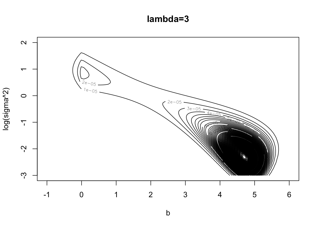
However, a slight change in lambda produces a more similar plot. It could just be that appearance is sensitive to details of how the contour plot is produced.
for(i in 1:length(b)){
  for(j in 1:length(ls2)){
    z[i,j] = post(exp(ls2[j]),b[i],lambda=3.5)
  }
}
contour(b,ls2,z,nlevels = 20,main="lambda=3.5",xlab="b",ylab="log(sigma^2)")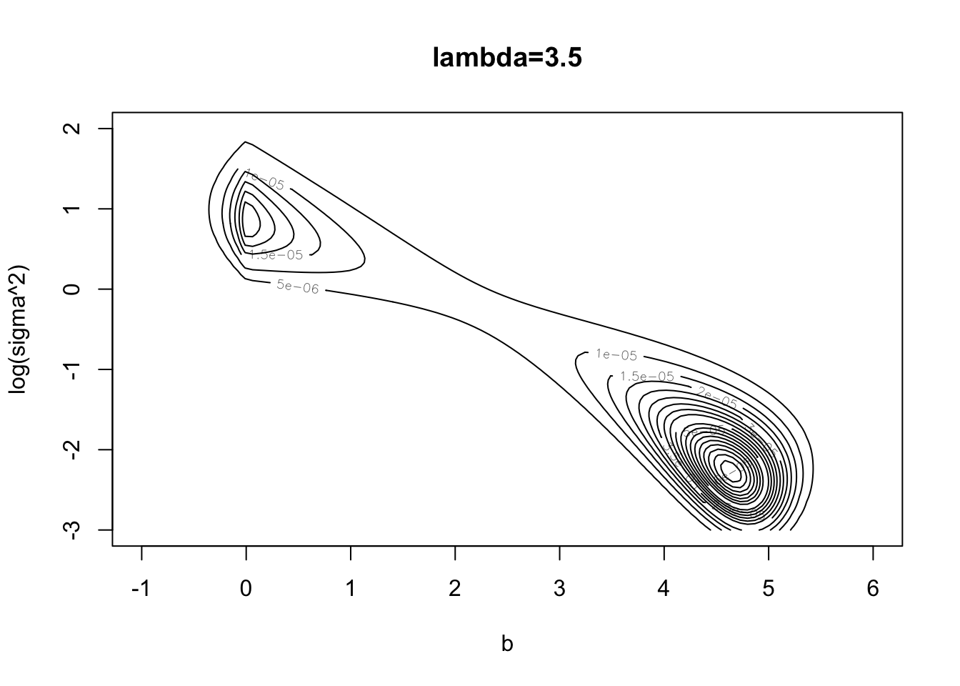
In sigma space
I was interested to see how the picture changes if we plot in sigma space instead of log(sigma). It is still bimodal.
contour(b,exp(ls2),z,nlevels = 20, main="lambda=3.5",xlab="b",ylab="sigma^2")
Scaled prior
Here we change so that the prior on \(b\) is scaled by \(\sigma\).
post2 = function(s2, b, yty=26, xtx=1, xty=5, n=10, lambda=3){
  (1/s2) * ((s2)^(-(n-1)/2)) * exp(-0.5*(1/s2)*(yty+b^2*xtx-2*xty*b) - (lambda/sqrt(s2))*abs(b) )
}

z2 = matrix(0,nrow=100, ncol=100)
for(i in 1:length(b)){
  for(j in 1:length(ls2)){
    z2[i,j] = post2(exp(ls2[j]),b[i],lambda=3.5)
  }
}
contour(b,ls2,z2)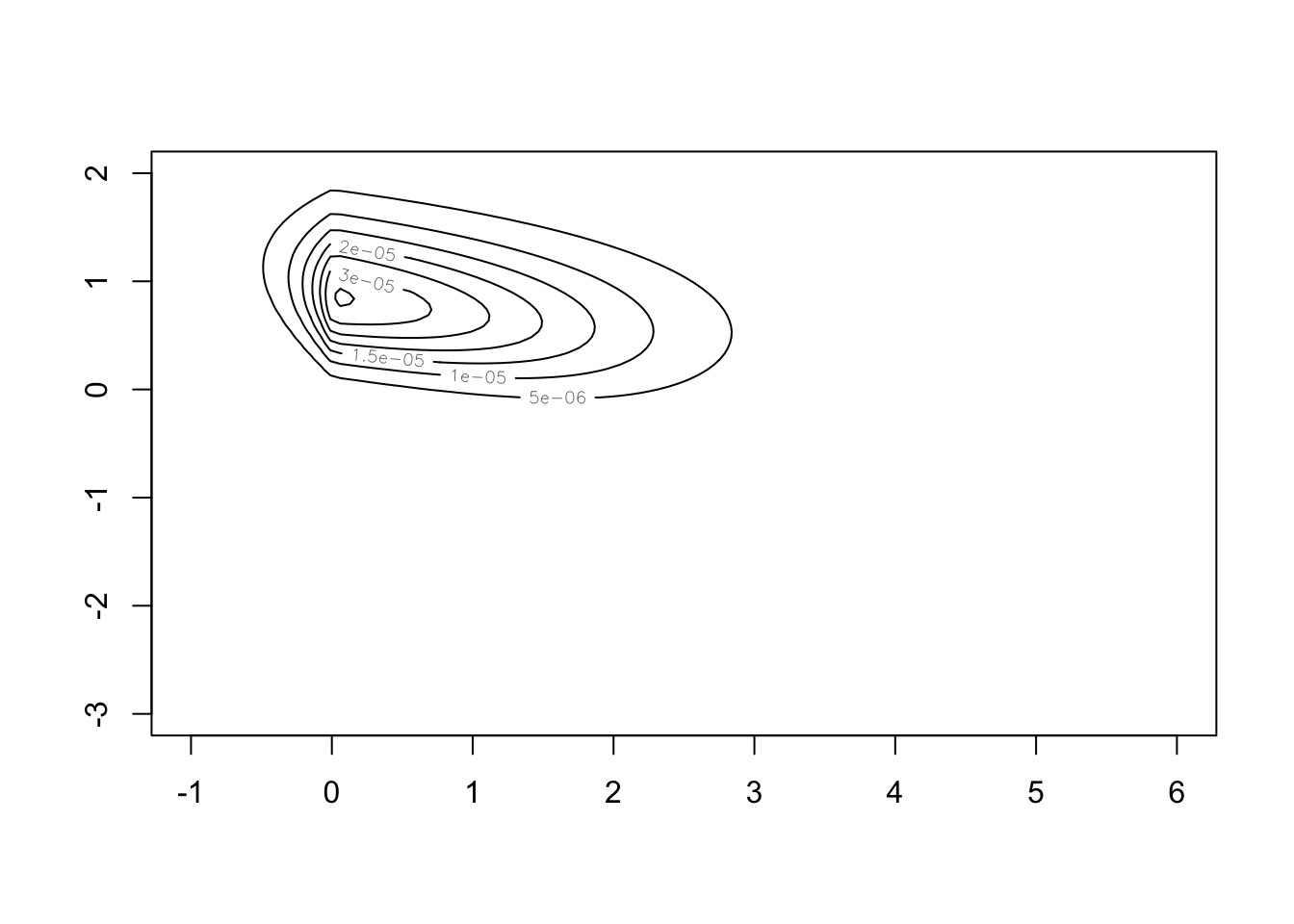
And try with some other lambda values:
for(i in 1:length(b)){
  for(j in 1:length(ls2)){
    z2[i,j] = post2(exp(ls2[j]),b[i],lambda=1)
  }
}
contour(b,ls2,z2,main="lambda=1",xlab="b",ylab="log(sigma^2)")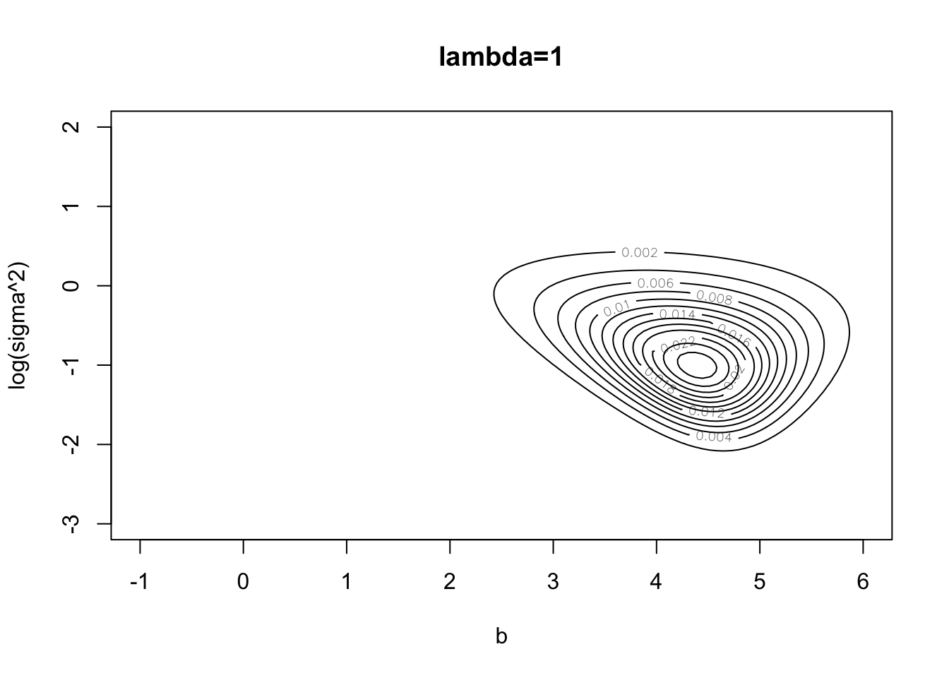
contour(b,exp(ls2),z2,main="lambda=1", ,xlab="b",ylab="sigma^2")
for(i in 1:length(b)){
  for(j in 1:length(ls2)){
    z2[i,j] = post2(exp(ls2[j]),b[i],lambda=1.5)
  }
}
contour(b,ls2,z2,main="lambda=1.5",xlab="b",ylab="log(sigma^2)")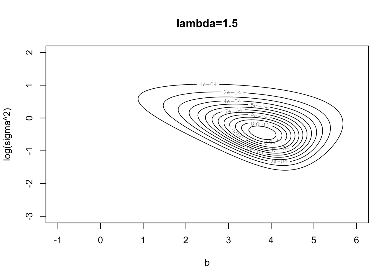
contour(b,exp(ls2),z2,main="lambda=1.5", ,xlab="b",ylab="sigma^2")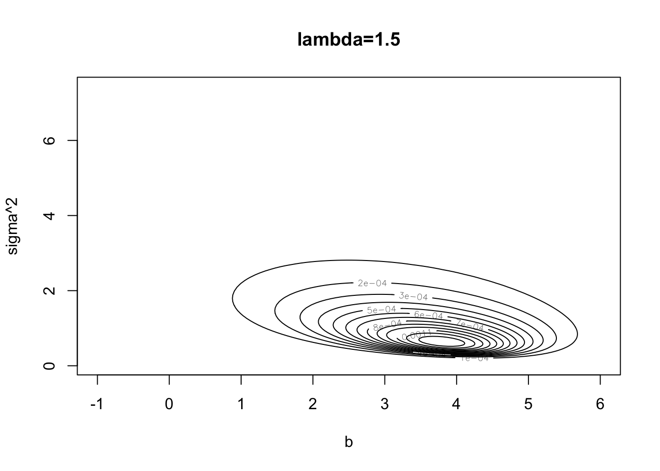
for(i in 1:length(b)){
  for(j in 1:length(ls2)){
    z2[i,j] = post2(exp(ls2[j]),b[i],lambda=2.5)
  }
}
contour(b,ls2,z2,main="lambda=2.5",xlab="b",ylab="log(sigma^2)")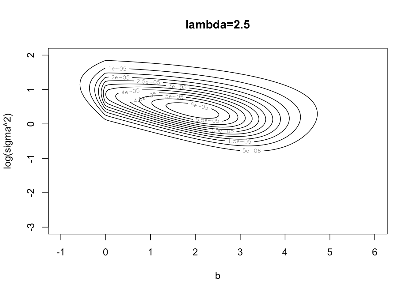
contour(b,exp(ls2),z2,main="lambda=2.5", ,xlab="b",ylab="sigma^2")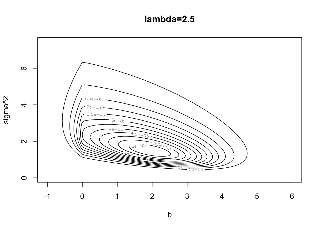
sessionInfo()R version 3.6.0 (2019-04-26)
Platform: x86_64-apple-darwin15.6.0 (64-bit)
Running under: macOS Mojave 10.14.6
Matrix products: default
BLAS: /Library/Frameworks/R.framework/Versions/3.6/Resources/lib/libRblas.0.dylib
LAPACK: /Library/Frameworks/R.framework/Versions/3.6/Resources/lib/libRlapack.dylib
locale:
[1] en_US.UTF-8/en_US.UTF-8/en_US.UTF-8/C/en_US.UTF-8/en_US.UTF-8
attached base packages:
[1] stats graphics grDevices utils datasets methods base
loaded via a namespace (and not attached):
[1] workflowr_1.6.1 Rcpp_1.0.4.6 rprojroot_1.3-2 digest_0.6.25
[5] later_1.0.0 R6_2.4.1 backports_1.1.5 git2r_0.26.1
[9] magrittr_1.5 evaluate_0.14 stringi_1.4.6 rlang_0.4.5
[13] fs_1.3.2 promises_1.1.0 whisker_0.4 rmarkdown_2.1
[17] tools_3.6.0 stringr_1.4.0 glue_1.4.0 httpuv_1.5.2
[21] xfun_0.12 yaml_2.2.1 compiler_3.6.0 htmltools_0.4.0
[25] knitr_1.28