ebnm_binormal

Last updated: 2025-03-12

Checks: 7 0

Knit directory: misc/analysis/

This reproducible R Markdown analysis was created with workflowr (version 1.7.1). The Checks tab describes the reproducibility checks that were applied when the results were created. The Past versions tab lists the development history.

R Markdown file: up-to-date

Great! Since the R Markdown file has been committed to the Git repository, you know the exact version of the code that produced these results.

Environment: empty

Great job! The global environment was empty. Objects defined in the global environment can affect the analysis in your R Markdown file in unknown ways. For reproduciblity it’s best to always run the code in an empty environment.

Seed: set.seed(1)

The command set.seed(1) was run prior to running the code in the R Markdown file. Setting a seed ensures that any results that rely on randomness, e.g. subsampling or permutations, are reproducible.

Session information: recorded

Great job! Recording the operating system, R version, and package versions is critical for reproducibility.

Cache: none

Nice! There were no cached chunks for this analysis, so you can be confident that you successfully produced the results during this run.

File paths: relative

Great job! Using relative paths to the files within your workflowr project makes it easier to run your code on other machines.

Repository version: 0be1b11

Great! You are using Git for version control. Tracking code development and connecting the code version to the results is critical for reproducibility.

The results in this page were generated with repository version 0be1b11. See the Past versions tab to see a history of the changes made to the R Markdown and HTML files.

Note that you need to be careful to ensure that all relevant files for the analysis have been committed to Git prior to generating the results (you can use wflow_publish or wflow_git_commit). workflowr only checks the R Markdown file, but you know if there are other scripts or data files that it depends on. Below is the status of the Git repository when the results were generated:


Ignored files:
    Ignored:    .DS_Store
    Ignored:    .Rhistory
    Ignored:    .Rproj.user/
    Ignored:    analysis/.RData
    Ignored:    analysis/.Rhistory
    Ignored:    analysis/ALStruct_cache/
    Ignored:    data/.Rhistory
    Ignored:    data/methylation-data-for-matthew.rds
    Ignored:    data/pbmc/
    Ignored:    data/pbmc_purified.RData

Untracked files:
    Untracked:  .dropbox
    Untracked:  Icon
    Untracked:  analysis/GHstan.Rmd
    Untracked:  analysis/GTEX-cogaps.Rmd
    Untracked:  analysis/PACS.Rmd
    Untracked:  analysis/Rplot.png
    Untracked:  analysis/SPCAvRP.rmd
    Untracked:  analysis/abf_comparisons.Rmd
    Untracked:  analysis/admm_02.Rmd
    Untracked:  analysis/admm_03.Rmd
    Untracked:  analysis/bispca.Rmd
    Untracked:  analysis/cache/
    Untracked:  analysis/cholesky.Rmd
    Untracked:  analysis/compare-transformed-models.Rmd
    Untracked:  analysis/cormotif.Rmd
    Untracked:  analysis/cp_ash.Rmd
    Untracked:  analysis/eQTL.perm.rand.pdf
    Untracked:  analysis/eb_prepilot.Rmd
    Untracked:  analysis/eb_var.Rmd
    Untracked:  analysis/ebpmf1.Rmd
    Untracked:  analysis/ebpmf_sla_text.Rmd
    Untracked:  analysis/ebpower.Rmd
    Untracked:  analysis/ebspca_sims.Rmd
    Untracked:  analysis/explore_psvd.Rmd
    Untracked:  analysis/fa_check_identify.Rmd
    Untracked:  analysis/fa_iterative.Rmd
    Untracked:  analysis/flash_cov_overlapping_groups_init.Rmd
    Untracked:  analysis/flash_test_tree.Rmd
    Untracked:  analysis/flashier_newgroups.Rmd
    Untracked:  analysis/flashier_nmf_triples.Rmd
    Untracked:  analysis/flashier_pbmc.Rmd
    Untracked:  analysis/flashier_snn_shifted_prior.Rmd
    Untracked:  analysis/greedy_ebpmf_exploration_00.Rmd
    Untracked:  analysis/ieQTL.perm.rand.pdf
    Untracked:  analysis/lasso_em_03.Rmd
    Untracked:  analysis/m6amash.Rmd
    Untracked:  analysis/mash_bhat_z.Rmd
    Untracked:  analysis/mash_ieqtl_permutations.Rmd
    Untracked:  analysis/methylation_example.Rmd
    Untracked:  analysis/mixsqp.Rmd
    Untracked:  analysis/mr.ash_lasso_init.Rmd
    Untracked:  analysis/mr.mash.test.Rmd
    Untracked:  analysis/mr_ash_modular.Rmd
    Untracked:  analysis/mr_ash_parameterization.Rmd
    Untracked:  analysis/mr_ash_ridge.Rmd
    Untracked:  analysis/mv_gaussian_message_passing.Rmd
    Untracked:  analysis/nejm.Rmd
    Untracked:  analysis/nmf_bg.Rmd
    Untracked:  analysis/nonneg_underapprox.Rmd
    Untracked:  analysis/normal_conditional_on_r2.Rmd
    Untracked:  analysis/normalize.Rmd
    Untracked:  analysis/pbmc.Rmd
    Untracked:  analysis/pca_binary_weighted.Rmd
    Untracked:  analysis/pca_l1.Rmd
    Untracked:  analysis/poisson_nmf_approx.Rmd
    Untracked:  analysis/poisson_shrink.Rmd
    Untracked:  analysis/poisson_transform.Rmd
    Untracked:  analysis/qrnotes.txt
    Untracked:  analysis/ridge_iterative_02.Rmd
    Untracked:  analysis/ridge_iterative_splitting.Rmd
    Untracked:  analysis/samps/
    Untracked:  analysis/sc_bimodal.Rmd
    Untracked:  analysis/shrinkage_comparisons_changepoints.Rmd
    Untracked:  analysis/susie_cov.Rmd
    Untracked:  analysis/susie_en.Rmd
    Untracked:  analysis/susie_z_investigate.Rmd
    Untracked:  analysis/svd-timing.Rmd
    Untracked:  analysis/temp.RDS
    Untracked:  analysis/temp.Rmd
    Untracked:  analysis/test-figure/
    Untracked:  analysis/test.Rmd
    Untracked:  analysis/test.Rpres
    Untracked:  analysis/test.md
    Untracked:  analysis/test_qr.R
    Untracked:  analysis/test_sparse.Rmd
    Untracked:  analysis/tree_dist_top_eigenvector.Rmd
    Untracked:  analysis/z.txt
    Untracked:  code/multivariate_testfuncs.R
    Untracked:  code/rqb.hacked.R
    Untracked:  data/4matthew/
    Untracked:  data/4matthew2/
    Untracked:  data/E-MTAB-2805.processed.1/
    Untracked:  data/ENSG00000156738.Sim_Y2.RDS
    Untracked:  data/GDS5363_full.soft.gz
    Untracked:  data/GSE41265_allGenesTPM.txt
    Untracked:  data/Muscle_Skeletal.ACTN3.pm1Mb.RDS
    Untracked:  data/P.rds
    Untracked:  data/Thyroid.FMO2.pm1Mb.RDS
    Untracked:  data/bmass.HaemgenRBC2016.MAF01.Vs2.MergedDataSources.200kRanSubset.ChrBPMAFMarkerZScores.vs1.txt.gz
    Untracked:  data/bmass.HaemgenRBC2016.Vs2.NewSNPs.ZScores.hclust.vs1.txt
    Untracked:  data/bmass.HaemgenRBC2016.Vs2.PreviousSNPs.ZScores.hclust.vs1.txt
    Untracked:  data/eb_prepilot/
    Untracked:  data/finemap_data/fmo2.sim/b.txt
    Untracked:  data/finemap_data/fmo2.sim/dap_out.txt
    Untracked:  data/finemap_data/fmo2.sim/dap_out2.txt
    Untracked:  data/finemap_data/fmo2.sim/dap_out2_snp.txt
    Untracked:  data/finemap_data/fmo2.sim/dap_out_snp.txt
    Untracked:  data/finemap_data/fmo2.sim/data
    Untracked:  data/finemap_data/fmo2.sim/fmo2.sim.config
    Untracked:  data/finemap_data/fmo2.sim/fmo2.sim.k
    Untracked:  data/finemap_data/fmo2.sim/fmo2.sim.k4.config
    Untracked:  data/finemap_data/fmo2.sim/fmo2.sim.k4.snp
    Untracked:  data/finemap_data/fmo2.sim/fmo2.sim.ld
    Untracked:  data/finemap_data/fmo2.sim/fmo2.sim.snp
    Untracked:  data/finemap_data/fmo2.sim/fmo2.sim.z
    Untracked:  data/finemap_data/fmo2.sim/pos.txt
    Untracked:  data/logm.csv
    Untracked:  data/m.cd.RDS
    Untracked:  data/m.cdu.old.RDS
    Untracked:  data/m.new.cd.RDS
    Untracked:  data/m.old.cd.RDS
    Untracked:  data/mainbib.bib.old
    Untracked:  data/mat.csv
    Untracked:  data/mat.txt
    Untracked:  data/mat_new.csv
    Untracked:  data/matrix_lik.rds
    Untracked:  data/paintor_data/
    Untracked:  data/running_data_chris.csv
    Untracked:  data/running_data_matthew.csv
    Untracked:  data/temp.txt
    Untracked:  data/y.txt
    Untracked:  data/y_f.txt
    Untracked:  data/zscore_jointLCLs_m6AQTLs_susie_eQTLpruned.rds
    Untracked:  data/zscore_jointLCLs_random.rds
    Untracked:  explore_udi.R
    Untracked:  output/fit.k10.rds
    Untracked:  output/fit.nn.pbmc.purified.rds
    Untracked:  output/fit.nn.rds
    Untracked:  output/fit.nn.s.001.rds
    Untracked:  output/fit.nn.s.01.rds
    Untracked:  output/fit.nn.s.1.rds
    Untracked:  output/fit.nn.s.10.rds
    Untracked:  output/fit.snn.s.001.rds
    Untracked:  output/fit.snn.s.01.nninit.rds
    Untracked:  output/fit.snn.s.01.rds
    Untracked:  output/fit.varbvs.RDS
    Untracked:  output/fit2.nn.pbmc.purified.rds
    Untracked:  output/glmnet.fit.RDS
    Untracked:  output/snn07.txt
    Untracked:  output/snn34.txt
    Untracked:  output/test.bv.txt
    Untracked:  output/test.gamma.txt
    Untracked:  output/test.hyp.txt
    Untracked:  output/test.log.txt
    Untracked:  output/test.param.txt
    Untracked:  output/test2.bv.txt
    Untracked:  output/test2.gamma.txt
    Untracked:  output/test2.hyp.txt
    Untracked:  output/test2.log.txt
    Untracked:  output/test2.param.txt
    Untracked:  output/test3.bv.txt
    Untracked:  output/test3.gamma.txt
    Untracked:  output/test3.hyp.txt
    Untracked:  output/test3.log.txt
    Untracked:  output/test3.param.txt
    Untracked:  output/test4.bv.txt
    Untracked:  output/test4.gamma.txt
    Untracked:  output/test4.hyp.txt
    Untracked:  output/test4.log.txt
    Untracked:  output/test4.param.txt
    Untracked:  output/test5.bv.txt
    Untracked:  output/test5.gamma.txt
    Untracked:  output/test5.hyp.txt
    Untracked:  output/test5.log.txt
    Untracked:  output/test5.param.txt

Unstaged changes:
    Modified:   .gitignore
    Modified:   analysis/flashier_log1p.Rmd
    Modified:   analysis/flashier_sla_text.Rmd
    Modified:   analysis/logistic_z_scores.Rmd
    Modified:   analysis/mr_ash_pen.Rmd
    Modified:   analysis/nmu_em.Rmd
    Modified:   analysis/susie_flash.Rmd
    Modified:   misc.Rproj

Note that any generated files, e.g. HTML, png, CSS, etc., are not included in this status report because it is ok for generated content to have uncommitted changes.

These are the previous versions of the repository in which changes were made to the R Markdown (analysis/ebnm_binormal.Rmd) and HTML (docs/ebnm_binormal.html) files. If you’ve configured a remote Git repository (see ?wflow_git_remote), click on the hyperlinks in the table below to view the files as they were in that past version.

File	Version	Author	Date	Message
Rmd	0be1b11	Matthew Stephens	2025-03-12	workflowr::wflow_publish("analysis/ebnm_binormal.Rmd")

library(ashr)

Introduction

I want to try implementing ebnm for a simple bimodal prior, consisting of a mixture of two normals, one with mean 0 and one with non-zero mean.

With this prior on \(\theta\), and \(x_i | \theta \sim N(\theta,s^2)\) we have the marginal likelihood \[x_i \sim \pi_0 N(0,\lambda^2 s_0^2+s^2) + \pi_1 N(\lambda, \lambda^2 s_0^2+s^2)\] where \(\lambda\) is a scaling factor to be estimated. For now I fix \(\pi_0=\pi_1=0.5\) and \(s_0\) to be smallish (it controls how bimodal this prior is).

Here I implement this marginal likelihood and its gradient (the latter obtained with the help of google AI).

dbinormal = function (x,s,s0,lambda,log=TRUE){
  pi0 = 0.5
  pi1 = 0.5
  s2 = s^2
  s02 = s0^2
  l0 = dnorm(x,0,sqrt(lambda^2 * s02 + s2),log=TRUE)
  l1 = dnorm(x,lambda,sqrt(lambda^2 * s02 + s2),log=TRUE)
  logsum = log(pi0*exp(l0) + pi1*exp(l1))
 
  m = pmax(l0,l1)
  logsum = m + log(pi0*exp(l0-m) + pi1*exp(l1-m))
  if (log) return(sum(logsum))
  else return(exp(sum(logsum)))
}

# Numerical gradient calculation
numerical_grad_dbinormal <- function(x, s, s0, lambda, delta = 1e-6) {
  f_plus <- dbinormal(x, s, s0, lambda + delta)
  f_minus <- dbinormal(x, s, s0, lambda - delta)
  return((f_plus - f_minus) / (2 * delta))
}

# Analytical gradient calculation
analytical_grad_dbinormal <- function(x, s, s0, lambda) {
  pi0 = 0.5
  pi1 = 0.5
  s2 = s^2
  s02 = s0^2
  sigma_lambda_sq <- lambda^2 * s02 + s2

  l0 <- dnorm(x, 0, sqrt(sigma_lambda_sq), log=TRUE)
  l1 <- dnorm(x, lambda, sqrt(sigma_lambda_sq), log=TRUE)

  dl0_dlambda <- -lambda * s02 / sigma_lambda_sq + lambda * s02 * x^2 / (sigma_lambda_sq^2)
  dl1_dlambda <- (x - lambda - lambda*s02) / sigma_lambda_sq + (x - lambda)^2 * lambda * s02 / (sigma_lambda_sq)^2

  # stably compute w0 and w1
  m <- pmax(l0, l1) # Find the maximum of l0 and l1
  w0 <- pi0 * exp(l0 - m) / (pi0 * exp(l0 - m) + pi1 * exp(l1 - m)) # Stable w0
  w1 <- pi1 * exp(l1 - m) / (pi0 * exp(l0 - m) + pi1 * exp(l1 - m)) # Stable w1


  grad_logsum <- w0 * dl0_dlambda + w1 * dl1_dlambda
  return(sum(grad_logsum)) 
}


# Example usage and comparison
x <- c(0.5,1,2)
s <- 1
s0 <- 0.5
lambda <- 1

num_grad <- numerical_grad_dbinormal(x, s, s0, lambda)
ana_grad <- analytical_grad_dbinormal(x, s, s0, lambda)

cat("Numerical Gradient:", num_grad, "\n")

Numerical Gradient: 0.1901379

cat("Analytical Gradient:", ana_grad, "\n")

Analytical Gradient: 0.1901379

Optimization using optim

Now I will try using optim to optimize this function. First I simulate some data.

# Simulate data
set.seed(1)
s = 1
s0 = 0.1
lambda = exp(4)

s2 = s^2
s02 = s0^2
n = 1000
x = c(rnorm(n,0,sqrt(lambda^2 * s02 + s2)),rnorm(n,lambda,sqrt(lambda^2 * s02 + s2)))
hist(x)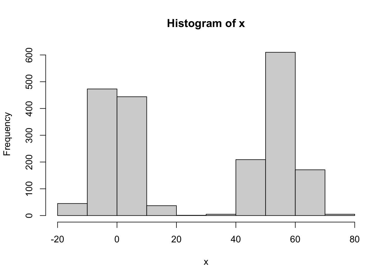

What I found is that it seems important to use a method that can be given bounds. (Note that (0,max(x)) are natural bounds). Eg Brents method, or L-BFGS-B. Using BFGS only works if you get the starting value right. (Possibly it works if you initialize at the upper bound, but it is hard to be confident that this will work generally).

objective_function <- function(lambda) {
  -dbinormal(x, s, s0, lambda) # Negative for minimization
}

gradient_function <- function(lambda) {
  -analytical_grad_dbinormal(x, s, s0, lambda) # Negative gradient for minimization
}

# optimization result initializing at true value
optim(par = lambda,
                      fn = objective_function,
                      gr = gradient_function,
                      method = "BFGS") # Using BFGS which uses gradient

$par
[1] 54.59053

$value
[1] 7727.426

$counts
function gradient 
      10        3 

$convergence
[1] 0

$message
NULL

#optim result initializing at 1
optim(par = 1,
                      fn = objective_function,
                      gr = gradient_function,
                      method = "BFGS") # Using BFGS which uses gradient

$par
[1] 83299.15

$value
[1] 21279.41

$counts
function gradient 
     100      100 

$convergence
[1] 1

$message
NULL

#optim result initializing at exp(3)
optim(par = exp(3),
                      fn = objective_function,
                      gr = gradient_function,
                      method = "BFGS") # Using BFGS which uses gradient

$par
[1] 16591.32

$value
[1] 18052.82

$counts
function gradient 
     100      100 

$convergence
[1] 1

$message
NULL

#optim result initializing at max(x)
optim(par = max(x),
                      fn = objective_function,
                      gr = gradient_function,
                      method = "BFGS") # Using BFGS which uses gradient

$par
[1] 54.59053

$value
[1] 7727.426

$counts
function gradient 
      24        8 

$convergence
[1] 0

$message
NULL

#optim result using L-BFGS-B
optim(par = 1,
                      fn = objective_function,
                      lower = 0, upper = max(x),
                      method = "L-BFGS-B")

$par
[1] 54.59053

$value
[1] 7727.426

$counts
function gradient 
       9        9 

$convergence
[1] 0

$message
[1] "CONVERGENCE: REL_REDUCTION_OF_F <= FACTR*EPSMCH"

#optim result using Brent
optim(par = 1,
                      fn = objective_function,
                      lower = 0, upper = max(x),
                      method = "Brent")

$par
[1] 54.59053

$value
[1] 7727.426

$counts
function gradient 
      NA       NA 

$convergence
[1] 0

$message
NULL

Here is a plot of the likelihood surface. You can see that if it starts at lambda too small then the gradient is huge, which I believe causes it to overshoot to crazy large values of lambda in methods where there is no upper bound. Maybe initializing at the upper bound (max(x)) will solve this, but it seems safer to use the bounded methods.

lambda = seq(1,100,length=100)
y = sapply(lambda,function(l) dbinormal(x,s,s0,l,log=TRUE))
plot(lambda,y,type="l")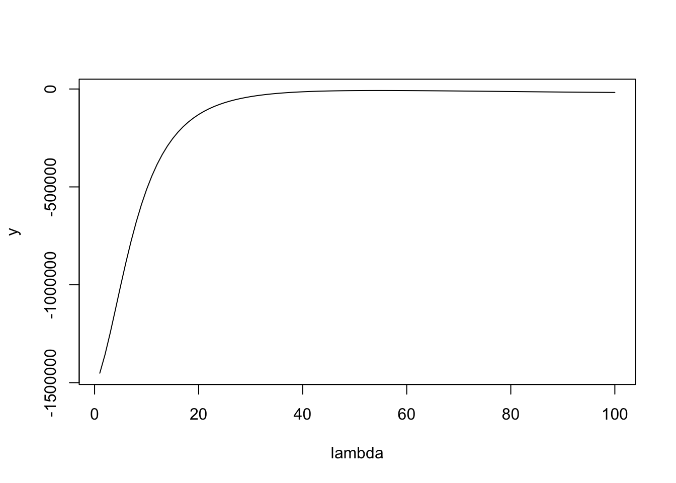

plot(lambda,y,type="l",ylim=c(-50000,0))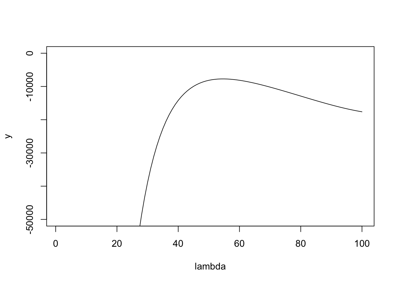

Here I use optimize (which is the same as optim with method=“Brent”) to find the maximum likelihood estimate of lambda. The following fixes s0=0.01. It may be worth investigating the idea of fixing s0 to be 0.01s to kind of fix the shrinkage behavior?

ebnm_binormal = function(x,s){
  s0 = 0.01
  lambda = optimize(function(lambda){-dbinormal(x,s,s0,lambda,log=TRUE)},
              lower = 0, upper = max(x))$minimum
  g = ashr::normalmix(pi=c(0.5,0.5), mean=c(0,lambda), sd=c(lambda * s0,lambda * s0))
  postmean = ashr::postmean(g,ashr::set_data(x,s))
  postsd = ashr::postsd(g,ashr::set_data(x,s))
  return(list(g = g, posterior = data.frame(mean=postmean,sd=postsd)))
}

res = ebnm_binormal(x,s)
plot(x,res$posterior$mean)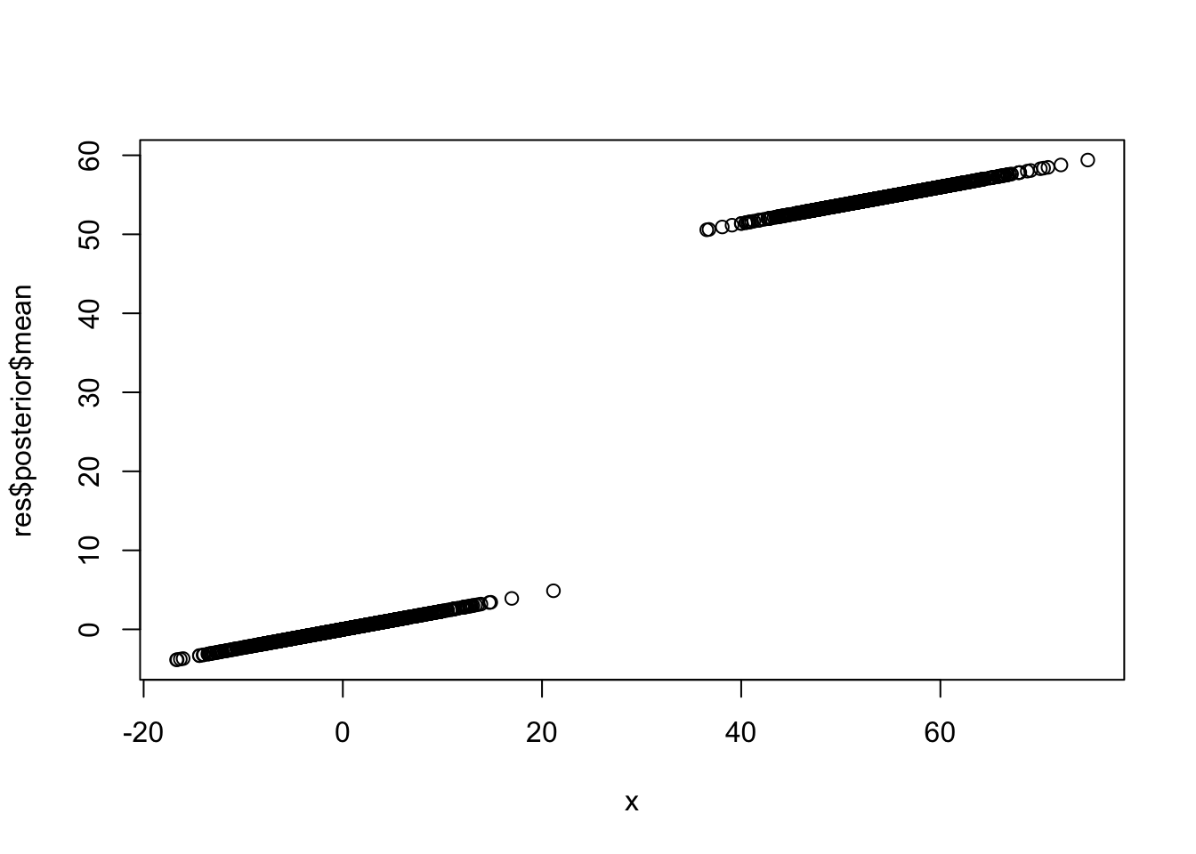

sessionInfo()

R version 4.4.2 (2024-10-31)
Platform: aarch64-apple-darwin20
Running under: macOS Sequoia 15.3.1

Matrix products: default
BLAS:   /Library/Frameworks/R.framework/Versions/4.4-arm64/Resources/lib/libRblas.0.dylib 
LAPACK: /Library/Frameworks/R.framework/Versions/4.4-arm64/Resources/lib/libRlapack.dylib;  LAPACK version 3.12.0

locale:
[1] en_US.UTF-8/en_US.UTF-8/en_US.UTF-8/C/en_US.UTF-8/en_US.UTF-8

time zone: America/Chicago
tzcode source: internal

attached base packages:
[1] stats     graphics  grDevices utils     datasets  methods   base     

other attached packages:
[1] ashr_2.2-63

loaded via a namespace (and not attached):
 [1] Matrix_1.7-2      jsonlite_1.8.9    compiler_4.4.2    promises_1.3.2   
 [5] Rcpp_1.0.14       stringr_1.5.1     git2r_0.35.0      later_1.4.1      
 [9] jquerylib_0.1.4   yaml_2.3.10       fastmap_1.2.0     lattice_0.22-6   
[13] R6_2.5.1          mixsqp_0.3-54     workflowr_1.7.1   knitr_1.49       
[17] tibble_3.2.1      rprojroot_2.0.4   bslib_0.9.0       pillar_1.10.1    
[21] rlang_1.1.5       cachem_1.1.0      SQUAREM_2021.1    stringi_1.8.4    
[25] httpuv_1.6.15     xfun_0.50         fs_1.6.5          sass_0.4.9       
[29] invgamma_1.1      truncnorm_1.0-9   cli_3.6.3         magrittr_2.0.3   
[33] digest_0.6.37     grid_4.4.2        irlba_2.3.5.1     rstudioapi_0.17.1
[37] lifecycle_1.0.4   vctrs_0.6.5       evaluate_1.0.3    glue_1.8.0       
[41] whisker_0.4.1     rmarkdown_2.29    tools_4.4.2       pkgconfig_2.0.3  
[45] htmltools_0.5.8.1

ebnm_binormal

Matthew Stephens

2025-03-12

Introduction

Optimization using optim