EB FastICA with Asymmetric Prior
Matthew Stephens (using Claude)
2026-07-29
Last updated: 2026-08-03
Checks: 7 0
Knit directory: misc/analysis/
This reproducible R Markdown analysis was created with workflowr (version 1.7.2). The Checks tab describes the reproducibility checks that were applied when the results were created. The Past versions tab lists the development history.
Great! Since the R Markdown file has been committed to the Git repository, you know the exact version of the code that produced these results.
Great job! The global environment was empty. Objects defined in the global environment can affect the analysis in your R Markdown file in unknown ways. For reproduciblity it’s best to always run the code in an empty environment.
The command set.seed(1) was run prior to running the
code in the R Markdown file. Setting a seed ensures that any results
that rely on randomness, e.g. subsampling or permutations, are
reproducible.
Great job! Recording the operating system, R version, and package versions is critical for reproducibility.
Nice! There were no cached chunks for this analysis, so you can be confident that you successfully produced the results during this run.
Great job! Using relative paths to the files within your workflowr project makes it easier to run your code on other machines.
Great! You are using Git for version control. Tracking code development and connecting the code version to the results is critical for reproducibility.
The results in this page were generated with repository version c09bf1b. See the Past versions tab to see a history of the changes made to the R Markdown and HTML files.
Note that you need to be careful to ensure that all relevant files for
the analysis have been committed to Git prior to generating the results
(you can use wflow_publish or
wflow_git_commit). workflowr only checks the R Markdown
file, but you know if there are other scripts or data files that it
depends on. Below is the status of the Git repository when the results
were generated:
Ignored files:
    Ignored:    .DS_Store
    Ignored:    .Rhistory
    Ignored:    .Rproj.user/
    Ignored:    .claude/
    Ignored:    GSE87571/
    Ignored:    analysis/.RData
    Ignored:    analysis/.Rhistory
    Ignored:    analysis/ALStruct_cache/
    Ignored:    analysis/ebproj_01.html
    Ignored:    data/.Rhistory
    Ignored:    data/methylation-data-for-matthew.rds
    Ignored:    data/pbmc/
    Ignored:    data/pbmc_purified.RData

Untracked files:
    Untracked:  .dropbox
    Untracked:  GSE41037/
    Untracked:  Icon
    Untracked:  Rplots.pdf
    Untracked:  analysis/GHstan.Rmd
    Untracked:  analysis/GTEX-cogaps.Rmd
    Untracked:  analysis/PACS.Rmd
    Untracked:  analysis/Rplot.png
    Untracked:  analysis/SPCAvRP.rmd
    Untracked:  analysis/abf_comparisons.Rmd
    Untracked:  analysis/admm_02.Rmd
    Untracked:  analysis/admm_03.Rmd
    Untracked:  analysis/bispca.Rmd
    Untracked:  analysis/cache/
    Untracked:  analysis/cholesky.Rmd
    Untracked:  analysis/compare-transformed-models.Rmd
    Untracked:  analysis/cormotif.Rmd
    Untracked:  analysis/cp_ash.Rmd
    Untracked:  analysis/eQTL.perm.rand.pdf
    Untracked:  analysis/eb_power2.Rmd
    Untracked:  analysis/eb_prepilot.Rmd
    Untracked:  analysis/eb_var.Rmd
    Untracked:  analysis/ebpmf1.Rmd
    Untracked:  analysis/ebpmf_sla_text.Rmd
    Untracked:  analysis/ebproj_01.Rmd
    Untracked:  analysis/ebproj_newton.Rmd
    Untracked:  analysis/ebspca_sims.Rmd
    Untracked:  analysis/explore_psvd.Rmd
    Untracked:  analysis/fa_check_identify.Rmd
    Untracked:  analysis/fa_iterative.Rmd
    Untracked:  analysis/fastica_asymmetric_02.Rmd
    Untracked:  analysis/fastica_heated.Rmd
    Untracked:  analysis/fastica_unwhitened.Rmd
    Untracked:  analysis/flash_cov_overlapping_groups_init.Rmd
    Untracked:  analysis/flash_test_tree.Rmd
    Untracked:  analysis/flashier_newgroups.Rmd
    Untracked:  analysis/flashier_nmf_triples.Rmd
    Untracked:  analysis/flashier_pbmc.Rmd
    Untracked:  analysis/flashier_snn_shifted_prior.Rmd
    Untracked:  analysis/greedy_ebpmf_exploration_00.Rmd
    Untracked:  analysis/ieQTL.perm.rand.pdf
    Untracked:  analysis/lasso_em_03.Rmd
    Untracked:  analysis/m6amash.Rmd
    Untracked:  analysis/mash_bhat_z.Rmd
    Untracked:  analysis/mash_ieqtl_permutations.Rmd
    Untracked:  analysis/matrix_beta.Rmd
    Untracked:  analysis/meth_flash_01.Rmd
    Untracked:  analysis/methylation_example.Rmd
    Untracked:  analysis/mixsqp.Rmd
    Untracked:  analysis/mr.ash_lasso_init.Rmd
    Untracked:  analysis/mr.mash.test.Rmd
    Untracked:  analysis/mr_ash_modular.Rmd
    Untracked:  analysis/mr_ash_parameterization.Rmd
    Untracked:  analysis/mr_ash_ridge.Rmd
    Untracked:  analysis/mv_gaussian_message_passing.Rmd
    Untracked:  analysis/nejm.Rmd
    Untracked:  analysis/nmf_bg.Rmd
    Untracked:  analysis/nonneg_underapprox.Rmd
    Untracked:  analysis/normal_conditional_on_r2.Rmd
    Untracked:  analysis/normalize.Rmd
    Untracked:  analysis/pbmc.Rmd
    Untracked:  analysis/pca_binary_weighted.Rmd
    Untracked:  analysis/pca_l1.Rmd
    Untracked:  analysis/poisson_nmf_approx.Rmd
    Untracked:  analysis/poisson_shrink.Rmd
    Untracked:  analysis/poisson_transform.Rmd
    Untracked:  analysis/qrnotes.txt
    Untracked:  analysis/ridge_iterative_02.Rmd
    Untracked:  analysis/ridge_iterative_splitting.Rmd
    Untracked:  analysis/samps/
    Untracked:  analysis/sc_bimodal.Rmd
    Untracked:  analysis/shrinkage_comparisons_changepoints.Rmd
    Untracked:  analysis/susie_cov.Rmd
    Untracked:  analysis/susie_en.Rmd
    Untracked:  analysis/susie_z_investigate.Rmd
    Untracked:  analysis/svd-timing.Rmd
    Untracked:  analysis/temp.RDS
    Untracked:  analysis/temp.Rmd
    Untracked:  analysis/test-figure/
    Untracked:  analysis/test.Rmd
    Untracked:  analysis/test.Rpres
    Untracked:  analysis/test.md
    Untracked:  analysis/test_qr.R
    Untracked:  analysis/test_sparse.Rmd
    Untracked:  analysis/tree_dist_top_eigenvector.Rmd
    Untracked:  analysis/z.txt
    Untracked:  code/coordinate_descent_symNMF.R
    Untracked:  code/multivariate_testfuncs.R
    Untracked:  code/rqb.hacked.R
    Untracked:  data/4matthew/
    Untracked:  data/4matthew2/
    Untracked:  data/E-MTAB-2805.processed.1/
    Untracked:  data/ENSG00000156738.Sim_Y2.RDS
    Untracked:  data/GDS5363_full.soft.gz
    Untracked:  data/GSE41265_allGenesTPM.txt
    Untracked:  data/Muscle_Skeletal.ACTN3.pm1Mb.RDS
    Untracked:  data/P.rds
    Untracked:  data/Thyroid.FMO2.pm1Mb.RDS
    Untracked:  data/bmass.HaemgenRBC2016.MAF01.Vs2.MergedDataSources.200kRanSubset.ChrBPMAFMarkerZScores.vs1.txt.gz
    Untracked:  data/bmass.HaemgenRBC2016.Vs2.NewSNPs.ZScores.hclust.vs1.txt
    Untracked:  data/bmass.HaemgenRBC2016.Vs2.PreviousSNPs.ZScores.hclust.vs1.txt
    Untracked:  data/eb_prepilot/
    Untracked:  data/finemap_data/fmo2.sim/b.txt
    Untracked:  data/finemap_data/fmo2.sim/dap_out.txt
    Untracked:  data/finemap_data/fmo2.sim/dap_out2.txt
    Untracked:  data/finemap_data/fmo2.sim/dap_out2_snp.txt
    Untracked:  data/finemap_data/fmo2.sim/dap_out_snp.txt
    Untracked:  data/finemap_data/fmo2.sim/data
    Untracked:  data/finemap_data/fmo2.sim/fmo2.sim.config
    Untracked:  data/finemap_data/fmo2.sim/fmo2.sim.k
    Untracked:  data/finemap_data/fmo2.sim/fmo2.sim.k4.config
    Untracked:  data/finemap_data/fmo2.sim/fmo2.sim.k4.snp
    Untracked:  data/finemap_data/fmo2.sim/fmo2.sim.ld
    Untracked:  data/finemap_data/fmo2.sim/fmo2.sim.snp
    Untracked:  data/finemap_data/fmo2.sim/fmo2.sim.z
    Untracked:  data/finemap_data/fmo2.sim/pos.txt
    Untracked:  data/logm.csv
    Untracked:  data/m.cd.RDS
    Untracked:  data/m.cdu.old.RDS
    Untracked:  data/m.new.cd.RDS
    Untracked:  data/m.old.cd.RDS
    Untracked:  data/mainbib.bib.old
    Untracked:  data/mat.csv
    Untracked:  data/mat.txt
    Untracked:  data/mat_new.csv
    Untracked:  data/matrix_lik.rds
    Untracked:  data/paintor_data/
    Untracked:  data/running_data_chris.csv
    Untracked:  data/running_data_matthew.csv
    Untracked:  data/temp.txt
    Untracked:  data/y.txt
    Untracked:  data/y_f.txt
    Untracked:  data/zscore_jointLCLs_m6AQTLs_susie_eQTLpruned.rds
    Untracked:  data/zscore_jointLCLs_random.rds
    Untracked:  explore_udi.R
    Untracked:  output/fit.k10.rds
    Untracked:  output/fit.nn.pbmc.purified.rds
    Untracked:  output/fit.nn.rds
    Untracked:  output/fit.nn.s.001.rds
    Untracked:  output/fit.nn.s.01.rds
    Untracked:  output/fit.nn.s.1.rds
    Untracked:  output/fit.nn.s.10.rds
    Untracked:  output/fit.snn.s.001.rds
    Untracked:  output/fit.snn.s.01.nninit.rds
    Untracked:  output/fit.snn.s.01.rds
    Untracked:  output/fit.varbvs.RDS
    Untracked:  output/fit2.nn.pbmc.purified.rds
    Untracked:  output/glmnet.fit.RDS
    Untracked:  output/snn07.txt
    Untracked:  output/snn34.txt
    Untracked:  output/test.bv.txt
    Untracked:  output/test.gamma.txt
    Untracked:  output/test.hyp.txt
    Untracked:  output/test.log.txt
    Untracked:  output/test.param.txt
    Untracked:  output/test2.bv.txt
    Untracked:  output/test2.gamma.txt
    Untracked:  output/test2.hyp.txt
    Untracked:  output/test2.log.txt
    Untracked:  output/test2.param.txt
    Untracked:  output/test3.bv.txt
    Untracked:  output/test3.gamma.txt
    Untracked:  output/test3.hyp.txt
    Untracked:  output/test3.log.txt
    Untracked:  output/test3.param.txt
    Untracked:  output/test4.bv.txt
    Untracked:  output/test4.gamma.txt
    Untracked:  output/test4.hyp.txt
    Untracked:  output/test4.log.txt
    Untracked:  output/test4.param.txt
    Untracked:  output/test5.bv.txt
    Untracked:  output/test5.gamma.txt
    Untracked:  output/test5.hyp.txt
    Untracked:  output/test5.log.txt
    Untracked:  output/test5.param.txt

Unstaged changes:
    Modified:   .gitignore
    Modified:   analysis/eb_snmu.Rmd
    Modified:   analysis/ebnm_binormal.Rmd
    Modified:   analysis/ebpower.Rmd
    Modified:   analysis/flashier_log1p.Rmd
    Modified:   analysis/flashier_sla_text.Rmd
    Modified:   analysis/logistic_z_scores.Rmd
    Modified:   analysis/mr_ash_pen.Rmd
    Modified:   analysis/nmu_em.Rmd
    Modified:   analysis/susie_flash.Rmd
    Modified:   analysis/tap_free_energy.Rmd
    Modified:   misc.Rproj
Note that any generated files, e.g. HTML, png, CSS, etc., are not included in this status report because it is ok for generated content to have uncommitted changes.
These are the previous versions of the repository in which changes were
made to the R Markdown (analysis/fastICA_asymmetric.Rmd)
and HTML (docs/fastICA_asymmetric.html) files. If you’ve
configured a remote Git repository (see ?wflow_git_remote),
click on the hyperlinks in the table below to view the files as they
were in that past version.
| File | Version | Author | Date | Message |
|---|---|---|---|---|
| Rmd | c09bf1b | Matthew Stephens | 2026-08-03 | workflowr::wflow_publish("analysis/fastICA_asymmetric.Rmd") |
| html | 0146cc1 | Matthew Stephens | 2026-07-30 | Publish fastICA_asymmetric: sorted-obj plots and objective diagnostics |
| Rmd | 4276a57 | Matthew Stephens | 2026-07-30 | Explain objective mismatch between asymmetric and log-cosh for symmetric source |
| html | 4276a57 | Matthew Stephens | 2026-07-30 | Explain objective mismatch between asymmetric and log-cosh for symmetric source |
| Rmd | b8658c2 | Matthew Stephens | 2026-07-29 | Add sorted-objective plots for all examples; fix Gaussian baseline text |
| html | b8658c2 | Matthew Stephens | 2026-07-29 | Add sorted-objective plots for all examples; fix Gaussian baseline text |
| Rmd | 636f7d0 | Matthew Stephens | 2026-07-29 | Add sorted-objective plots to assess objective as a source-selection criterion |
| html | 636f7d0 | Matthew Stephens | 2026-07-29 | Add sorted-objective plots to assess objective as a source-selection criterion |
| Rmd | a875fd7 | Matthew Stephens | 2026-07-29 | Clarify log-cosh local-minimum interpretation for p=0.1 nine-groups case |
| html | a875fd7 | Matthew Stephens | 2026-07-29 | Clarify log-cosh local-minimum interpretation for p=0.1 nine-groups case |
| Rmd | 43a0155 | Matthew Stephens | 2026-07-29 | Add p=0.1 to 9-groups and p=0.2 to single-source k=20 tests |
| html | 43a0155 | Matthew Stephens | 2026-07-29 | Add p=0.1 to 9-groups and p=0.2 to single-source k=20 tests |
| Rmd | 9878c1e | Matthew Stephens | 2026-07-29 | Add log-cosh trace Hessian comparison across all tests |
| html | 9878c1e | Matthew Stephens | 2026-07-29 | Add log-cosh trace Hessian comparison across all tests |
| Rmd | 2f935c7 | Matthew Stephens | 2026-07-29 | Match k=20 p=0.5 simulation exactly to ebproj_newton (set.seed(10), n=200, p=1000) |
| html | 2f935c7 | Matthew Stephens | 2026-07-29 | Match k=20 p=0.5 simulation exactly to ebproj_newton (set.seed(10), n=200, p=1000) |
| Rmd | 5df95fa | Matthew Stephens | 2026-07-29 | Add single-source k=20 tests (p=0.5 and p=0.1) |
| html | 5df95fa | Matthew Stephens | 2026-07-29 | Add single-source k=20 tests (p=0.5 and p=0.1) |
| Rmd | 7686e79 | Matthew Stephens | 2026-07-29 | Add trace Hessian approximation to asymmetric fastICA |
| html | 7686e79 | Matthew Stephens | 2026-07-29 | Add trace Hessian approximation to asymmetric fastICA |
| Rmd | f421e5c | Matthew Stephens | 2026-07-29 | Add warm-start comparison to 9-groups test |
| html | f421e5c | Matthew Stephens | 2026-07-29 | Add warm-start comparison to 9-groups test |
| Rmd | d03ae26 | Matthew Stephens | 2026-07-29 | Add warm-start comparison for symmetric sources |
| html | d03ae26 | Matthew Stephens | 2026-07-29 | Add warm-start comparison for symmetric sources |
| Rmd | 008f9d4 | Matthew Stephens | 2026-07-29 | Add EB fastICA with asymmetric prior |
| html | 008f9d4 | Matthew Stephens | 2026-07-29 | Add EB fastICA with asymmetric prior |
Introduction
I gave Claude the following outline (generated in conversation with Gemini) plus some pseudo code also generated by Gemini. Most of the rest of the text and code was created by Claude, with some light editing from me. It is far from a polished document and I did not edit all the AI-generated text, so take some of the comments with a pinch of salt.
The basic idea was to optimize the function \(J(w, cg_p; \sigma^2=cs)\) subject to \(w'Dw=1\). Here \(s\) is the standard deviation of the data (\(=1\) for whitened data), \(g_p\) is a binary prior with up-probability \(p\), scaled to have variance 1, and \(cg_p\) denotes this prior scaled by \(c\) (so with variance \(c^2\)).
Fixing \(\sigma^2 = cs\) ensures that at \(p=0.5\) the optimization of \(J\) is equivalent to fastICA. I consider \(c\) to be either fixed to 1 (Gemini’s suggestion) or the inverse of the “golden ratio”. The latter ensures that \(var(g) + \sigma^2 = s^2\). I decided that fixing both \(c\) and \(\sigma^2\) ultimately is not the way to go: it does not allow the objective function to be sufficiently binary. I learned some things from this experiment, but ultimately it can probably be ignored as I hope that subsequent investigations will be better and more polished. Consider it a quick first try.
1. Motivation
The standard fastICA algorithm is widely utilized for blind source separation, predominantly employing the symmetric \(\log \cosh\) contrast function. This contrast function is mathematically equivalent to assuming a symmetric, binary prior on the underlying independent components.
The objective of this project is to generalize the fastICA framework to actively isolate skewed (asymmetric) independent components. We achieve this by relaxing the assumed symmetric prior to an asymmetric Rademacher distribution. To ensure the algorithm remains scale-invariant and highly stable, we must carefully constrain the variance parameters of the generative model to match the empirical variance of the sphered data.
2. The Generative Model
Let the sphered (whitened) data matrix be \(Y \in \mathbb{R}^{n \times m}\). Algebraically, we can express this decomposition as \(Y = U D\), where \(D = s\sqrt{n}I_m\) (for whitened data, \(s=1\)) and \(U \in \mathbb{R}^{n \times m}\) has orthonormal columns (\(U^T U = I_m\)). This ensures the empirical covariance is \(\frac{1}{n}Y^T Y = s^2 I_m\), meaning the variance of any 1D projection \(x = Yw\) (strictly constraining the rotation vector such that \(w^T w = 1\)) is exactly \(s^2\).
We assume the 1D projection \(x\) is generated by a signal corrupted by Gaussian noise: \(x = v + \epsilon\), where \(\epsilon \sim \mathcal{N}(0, \sigma^2)\). The signal \(v\) is drawn from an asymmetric Rademacher distribution with variance \(c^2\) and an upper-state probability \(p\). To maintain a zero mean, the two support points are uniquely determined as: \[y_1 = c\sqrt{\frac{1-p}{p}} \quad \text{and} \quad y_0 = -c\sqrt{\frac{p}{1-p}}\]
3. Resolving Parameter Ambiguity
To preserve the robust, scale-invariant optimization landscape of traditional fastICA on data with variance \(s^2\), we must enforce a specific relationship between the prior scale \(c\), the noise variance \(\sigma^2\), and the empirical data scale \(s\): \[\sigma^2 = cs\] This constraint acts as a dynamic standardizer inside the log-partition function, ensuring the data is implicitly evaluated at unit variance (\(\frac{x}{s}\)). Crucially, because of this constraint, any choice of \(c\) will strictly recover standard fastICA when the prior is symmetric (\(p=0.5\)). With \(\sigma^2\) locked to \(cs\), we are left with the choice of the baseline scale parameter \(c\) for when \(p \neq 0.5\). We propose two theoretically justified default anchors:
- Option A: The M-Estimator Anchor (\(c = s\)) While any \(c\) recovers standard fastICA at \(p=0.5\), choosing \(c=s\) ensures that when asymmetry is introduced, the empirical data and the geometric skewness penalty are weighted equally (1-to-1). It is theoretically misspecified in variance (expecting a total generative variance of \(2s^2\)), but performs exceptionally well as a robust M-estimator by keeping the non-linearity centered optimally relative to the data spread.
- Option B: The Golden Ratio Anchor (\(c = 0.618s\)) This choice strictly matches the assumed generative variance to the empirical data variance. The total assumed variance is \(c^2 + \sigma^2\). If we demand \(c^2 + cs = s^2\), solving this quadratic yields \(c = s(\frac{\sqrt{5}-1}{2}) \approx 0.618s\). This specifies a model where approximately 38.2% of the energy is signal and 61.8% is noise, resulting in a slightly softer asymmetry penalty during optimization.
4. The Alternating Optimization Algorithm
We maximize the dual objective \(J(w, p; \sigma^2=cs)\) over both the vector \(w\) and the asymmetry parameter \(p\). For a fixed scale parameter \(c\), the total objective function evaluated over \(n\) data points \(x_i = (Yw)_i\) is defined as: \[J(w, p) = \frac{1}{n} \sum_{i=1}^n \left[ -\frac{c}{2s} + \log\left( p \exp\left(\frac{x_i y_1}{cs} - \frac{y_1^2}{2cs}\right) + (1-p) \exp\left(\frac{x_i y_0}{cs} - \frac{y_0^2}{2cs}\right) \right) \right]\] The algorithm alternates between updating \(w\) via gradient ascent on the score function, and updating \(p\) via a bounded 1D scalar optimization.
Claude’s Introduction
Standard fastICA maximizes the log-cosh contrast function, which is equivalent to assuming a symmetric binary (Rademacher) prior on the independent components. For sparse or skewed sources (e.g. indicator variables where the “on” fraction \(p \ll 0.5\)), the expected log-cosh contrast falls below the Gaussian baseline, causing fastICA to actively avoid the true source direction.
This analysis generalizes the framework to an asymmetric Rademacher prior parameterized by its up-probability \(p\). We alternate between:
- Updating the projection direction \(w\) via a Newton-like fixed-point step (for fixed \(p\)).
- Updating \(p\) by maximizing the marginal log-likelihood (for fixed \(w\)).
At \(p = 0.5\) the algorithm exactly reduces to standard log-cosh fastICA. Two scale anchors are compared:
- M-estimator (\(c = s\)): robust but slightly over-inflated variance.
- Golden-ratio (\(c \approx 0.618\,s\)): satisfies \(c^2 + cs = s^2\), so the assumed generative variance equals the empirical data variance.
Helpers
prewhiten = function(X, n.comp) {
  X = X - rowMeans(X)
  sqrt(ncol(X)) * t(svd(X)$v[, 1:n.comp])
}
Implementation
With \(\sigma^2 = cs\), the score function and its derivative are:
\[M(x) = \frac{y_1}{cs}\,\pi(x) + \frac{y_0}{cs}\,(1-\pi(x)), \qquad M'(x) = \frac{\pi(x)(1-\pi(x))}{s^2\,p(1-p)}\]
where \(\pi(x) = \sigma(\Delta(x))\) is the logistic sigmoid of
\[\Delta(x) = \frac{1}{\sqrt{p(1-p)}}\!\left(\frac{x}{s} - \frac{c\,(1-2p)}{2s\,\sqrt{p(1-p)}}\right) + \log\frac{p}{1-p}\]
and \(y_1 = c\sqrt{(1-p)/p} > 0\), \(y_0 = -c\sqrt{p/(1-p)} < 0\) are the prior support points.
asym_score = function(x, p, c, s) {
  y1     = c * sqrt((1-p)/p)
  y0     = -c * sqrt(p/(1-p))
  kappa3 = (1 - 2*p) / sqrt(p*(1-p))
  Delta  = (x/s - c*kappa3/(2*s)) / sqrt(p*(1-p)) + log(p/(1-p))
  pi_x   = plogis(Delta)
  list(
    M  = (y1/(c*s)) * pi_x + (y0/(c*s)) * (1 - pi_x),
    Mp = pi_x * (1 - pi_x) / (s^2 * p * (1-p))
  )
}
The marginal log-likelihood in \(p\) for fixed projections \(x = Yw\):
\[J(p) = \frac{1}{n}\sum_{i=1}^n \log\!\left( p\,e^{\,x_i y_1/(cs)\,-\,y_1^2/(2cs)} + (1-p)\,e^{\,x_i y_0/(cs)\,-\,y_0^2/(2cs)}\right)\]
asym_obj_p = function(p, x, c, s) {
  y1  = c * sqrt((1-p)/p)
  y0  = -c * sqrt(p/(1-p))
  a1  = x * y1/(c*s) - y1^2/(2*c*s)
  a0  = x * y0/(c*s) - y0^2/(2*c*s)
  lp  = log(p); l1p = log(1-p)
  m   = pmax(lp + a1, l1p + a0)
  mean(m + log(exp(lp + a1 - m) + exp(l1p + a0 - m)))
}
Two diagonal Hessian approximations are supported, following the notation in ebproj_newton:
- fastICA: \(\tilde H = \overline{M'(x)}\,\mathbf{I}\) — uniform sample weights.
- trace: \(\tilde H = c_\text{trace}\,\mathbf{I}\) where \(c_\text{trace} = \tfrac{1}{k}\sum_i M'(x_i)\,S_{ii}\) and \(S_{ii} = \tfrac{1}{n}\|Y_{:i}\|^2\) is the squared distance of sample \(i\) from the origin (with \(\sum_i S_{ii} = k\) for whitened data).
Both reduce to the same Newton fixed-point update structure: \[w \leftarrow \tfrac{1}{n}Y M(x) - \tilde H\,w, \qquad w \leftarrow w / \|w\|\]
fastica_asym_r1 = function(Y, s = 1, anchor = c("M", "golden"),
                            hess = c("fastICA", "trace"),
                            tol = 1e-6, max_iter = 500, eps = 0.01,
                            w_init = NULL) {
  anchor = match.arg(anchor)
  hess   = match.arg(hess)
  c      = if (anchor == "M") s else s * (sqrt(5)-1)/2
  m = nrow(Y); n = ncol(Y)
  S_diag = colSums(Y^2) / n   # S_ii = ||Y[:,i]||^2 / n  (sum = m)
  w = if (is.null(w_init)) rnorm(m) else w_init
  w = w / sqrt(sum(w^2))
  p = 0.5
  for (iter in seq_len(max_iter)) {
    w_old = w; p_old = p
    x  = as.vector(t(Y) %*% w)
    sc = asym_score(x, p, c, s)
    h  = if (hess == "trace") sum(sc$Mp * S_diag) / m else mean(sc$Mp)
    w  = as.vector(Y %*% sc$M) / n - h * w
    w  = w / sqrt(sum(w^2))
    x   = as.vector(t(Y) %*% w)
    opt = optimize(\(pp) asym_obj_p(pp, x, c, s), c(eps, 1-eps), maximum = TRUE)
    p   = opt$maximum
    if (1 - abs(sum(w * w_old)) < tol && abs(p - p_old) < tol) break
  }
  list(w = w, p = p, iter = iter, c = c)
}
Standard log-cosh fastICA for comparison:
fastica_r1update = function(X, w) {
  w = w / sqrt(sum(w^2))
  P  = t(X) %*% w
  G  = tanh(P); G2 = 1 - tanh(P)^2
  w  = X %*% G - mean(G2) * ncol(X) * w
  w / sqrt(sum(w^2))
}

fastica_r1update_trace = function(X, w, S_diag) {
  w = w / sqrt(sum(w^2))
  P  = t(X) %*% w
  G  = tanh(P); G2 = 1 - tanh(P)^2
  h  = sum(G2 * S_diag) / nrow(X)   # trace Hessian: Σ G2_i S_ii / k
  w  = as.vector(X %*% G) / ncol(X) - h * w
  w / sqrt(sum(w^2))
}

run_seeds_lc = function(Y, S_true, hess = "fastICA", n_seeds = 100, n_iter = 200) {
  maxcor = numeric(n_seeds)
  objs   = numeric(n_seeds)
  S_diag = colSums(Y^2) / ncol(Y)
  for (seed in seq_len(n_seeds)) {
    set.seed(seed)
    w = rnorm(nrow(Y))
    if (hess == "trace") {
      for (i in seq_len(n_iter)) w = fastica_r1update_trace(Y, w, S_diag)
    } else {
      for (i in seq_len(n_iter)) w = fastica_r1update(Y, w)
    }
    maxcor[seed] = max(abs(cor(t(S_true), t(Y) %*% w)))
    objs[seed]   = mean(log(cosh(as.vector(t(Y) %*% w))))
  }
  structure(maxcor, obj = objs)   # vector; objs accessible via attr(., "obj")
}

run_seeds_asym = function(Y, S_true, anchor, hess = "fastICA", n_seeds = 100) {
  maxcor = numeric(n_seeds); ps = numeric(n_seeds); objs = numeric(n_seeds)
  for (seed in seq_len(n_seeds)) {
    set.seed(seed)
    res = fastica_asym_r1(Y, anchor = anchor, hess = hess, w_init = rnorm(nrow(Y)))
    maxcor[seed] = max(abs(cor(t(S_true), t(Y) %*% res$w)))
    ps[seed]     = min(res$p, 1 - res$p)
    objs[seed]   = asym_obj_p(res$p, as.vector(t(Y) %*% res$w), res$c, 1)
  }
  list(maxcor = maxcor, p = ps, obj = objs)
}

# Warm-start variant: run log-cosh to convergence, then hand off to asymmetric
run_seeds_asym_warm = function(Y, S_true, anchor, hess = "fastICA", n_seeds = 100,
                                n_iter_lc = 200) {
  maxcor = numeric(n_seeds); ps = numeric(n_seeds); objs = numeric(n_seeds)
  for (seed in seq_len(n_seeds)) {
    set.seed(seed)
    w = rnorm(nrow(Y))
    for (i in seq_len(n_iter_lc)) w = fastica_r1update(Y, w)
    res = fastica_asym_r1(Y, anchor = anchor, hess = hess, w_init = w)
    maxcor[seed] = max(abs(cor(t(S_true), t(Y) %*% res$w)))
    ps[seed]     = min(res$p, 1 - res$p)
    objs[seed]   = asym_obj_p(res$p, as.vector(t(Y) %*% res$w), res$c, 1)
  }
  list(maxcor = maxcor, p = ps, obj = objs)
}

# Sort by |obj − Gaussian baseline| (most extreme first), colour by success
plot_obj_lc = function(lc_result, title, lc_gauss) {
  objs = attr(lc_result, "obj")
  succ = lc_result > 0.9
  ord  = order(abs(objs - lc_gauss), decreasing = TRUE)
  cols = ifelse(succ[ord], "steelblue", "tomato")
  plot(seq_along(objs), objs[ord],
       pch = 19, cex = 0.7, col = cols,
       xlab = "rank (1 = most extreme log-cosh)",
       ylab = "log-cosh objective",
       main = paste0(title, "\n(blue = found true source, red = not)"))
  abline(h = lc_gauss, lty = 2, col = "grey50")
  legend("topright", c("true source", "other", "Gaussian baseline"),
         pch = c(19, 19, NA), lty = c(NA, NA, 2),
         col = c("steelblue", "tomato", "grey50"), bty = "n", cex = 0.8)
}

plot_obj_asym = function(asym_result, title) {
  objs = asym_result$obj
  succ = asym_result$maxcor > 0.9
  ord  = order(objs, decreasing = TRUE)
  cols = ifelse(succ[ord], "steelblue", "tomato")
  plot(seq_along(objs), objs[ord],
       pch = 19, cex = 0.7, col = cols,
       xlab = "rank (1 = highest asymmetric objective)",
       ylab = "asymmetric log-likelihood",
       main = paste0(title, "\n(blue = found true source, red = not)"))
  legend("topright", c("true source", "other"),
         pch = 19, col = c("steelblue", "tomato"), bty = "n", cex = 0.8)
}
Sanity check: \(p = 0.5\) recovers log-cosh
At \(p = 0.5\), \(s = 1\): \(\Delta(x) = 2x\), \(\pi(x) = (1 + \tanh x)/2\), and \(M(x) = \tanh(x)\) — the standard fastICA score.
x_grid = seq(-3, 3, length.out = 300)
sc05   = asym_score(x_grid, p = 0.5, c = 1, s = 1)

plot(x_grid, sc05$M, type = "l", col = "steelblue", lwd = 2,
     xlab = "x", ylab = "M(x)",
     main = "Score function at p = 0.5 vs tanh(x)")
lines(x_grid, tanh(x_grid), col = "tomato", lty = 2, lwd = 2)
legend("topleft", c("asymmetric M(x), p = 0.5", "tanh(x)"),
       col = c("steelblue", "tomato"), lty = c(1, 2), lwd = 2, bty = "n")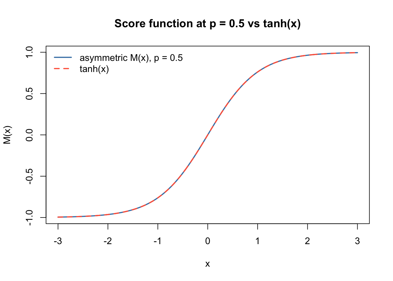
The curves are numerically identical.
Theoretical motivation
When does log-cosh fail? For a standardised binary source \((\text{Bernoulli}(p)\), zero mean, unit variance), the expected log-cosh contrast is:
expected_logcosh = function(p) {
  z1 =  sqrt((1-p)/p); z0 = -sqrt(p/(1-p))
  p * log(cosh(z1)) + (1-p) * log(cosh(z0))
}
lc_stable = function(z) abs(z) + log1p(exp(-2*abs(z))) - log(2)
lc_gauss  = integrate(\(z) lc_stable(z) * dnorm(z), -Inf, Inf)$value

pvec = seq(0.01, 0.99, by = 0.01)
lc   = sapply(pvec, expected_logcosh)

plot(pvec, lc, type = "l", col = "steelblue", lwd = 2,
     xlab = "p  (probability of positive state)",
     ylab = "E[log cosh(x)]",
     main = "Log-cosh contrast vs Gaussian baseline")
abline(h = lc_gauss, lty = 2, col = "grey40")
legend("top", c("E[log cosh], binary source", "Gaussian baseline"),
       col = c("steelblue", "grey40"), lty = c(1, 2), lwd = 2, bty = "n")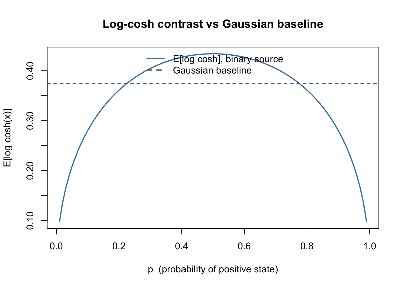
Standard fastICA with log-cosh actively avoids sources with $p < $ about \(0.25\) or \(p > 0.75\): the contrast falls below the Gaussian baseline, so the global maximum of \(E[\log\cosh]\) on the sphere is not at the true source. However, the true source direction can still be a local minimum, and the fixed-point iteration can converge there when \(p\) is small enough (see the \(p=0.1\) nine-groups result below).
Asymmetric objective for \(p_\text{true} = 0.2\)
The following plot shows the asymmetric objective (as a function of \(p\)) evaluated for a Rademacher source with \(p=0.2\) (blue) and a Gaussian source (grey dashed). At the true \(p\) the asymmetric source is higher; at \(p=0.5\) the Gaussian source is higher.
set.seed(42)
n_pop  = 100000
c_gr   = (sqrt(5) - 1) / 2   # golden-ratio anchor
z_02   = ifelse(runif(n_pop) < 0.2, sqrt(0.8/0.2), -sqrt(0.2/0.8))
z_N    = rnorm(n_pop)

p_grid      = seq(0.02, 0.98, by = 0.01)
obj_asym_02 = sapply(p_grid, \(p) asym_obj_p(p, z_02, c_gr, 1))
obj_asym_N  = sapply(p_grid, \(p) asym_obj_p(p, z_N,  c_gr, 1))

plot(p_grid, obj_asym_02, type = "l", col = "steelblue", lwd = 2,
     xlab = "test p  (optimization variable)",
     ylab = "E[asymmetric log-likelihood]",
     main = "Asymmetric objective: source p_true = 0.2  (golden-ratio anchor)")
lines(p_grid, obj_asym_N, col = "grey40", lty = 2, lwd = 2)
abline(v = 0.2, lty = 3, col = "tomato", lwd = 1.5)
abline(v = 0.5, lty = 3, col = "orange", lwd = 1.5)
legend("topright",
       c("asymm source (p_true = 0.2)", "Gaussian source", "p = 0.2", "p=0.5"),
       col = c("steelblue", "grey40", "tomato","orange"),
       lty = c(1, 2, 3,3), lwd = c(2, 2, 1.5,1.5), bty = "n")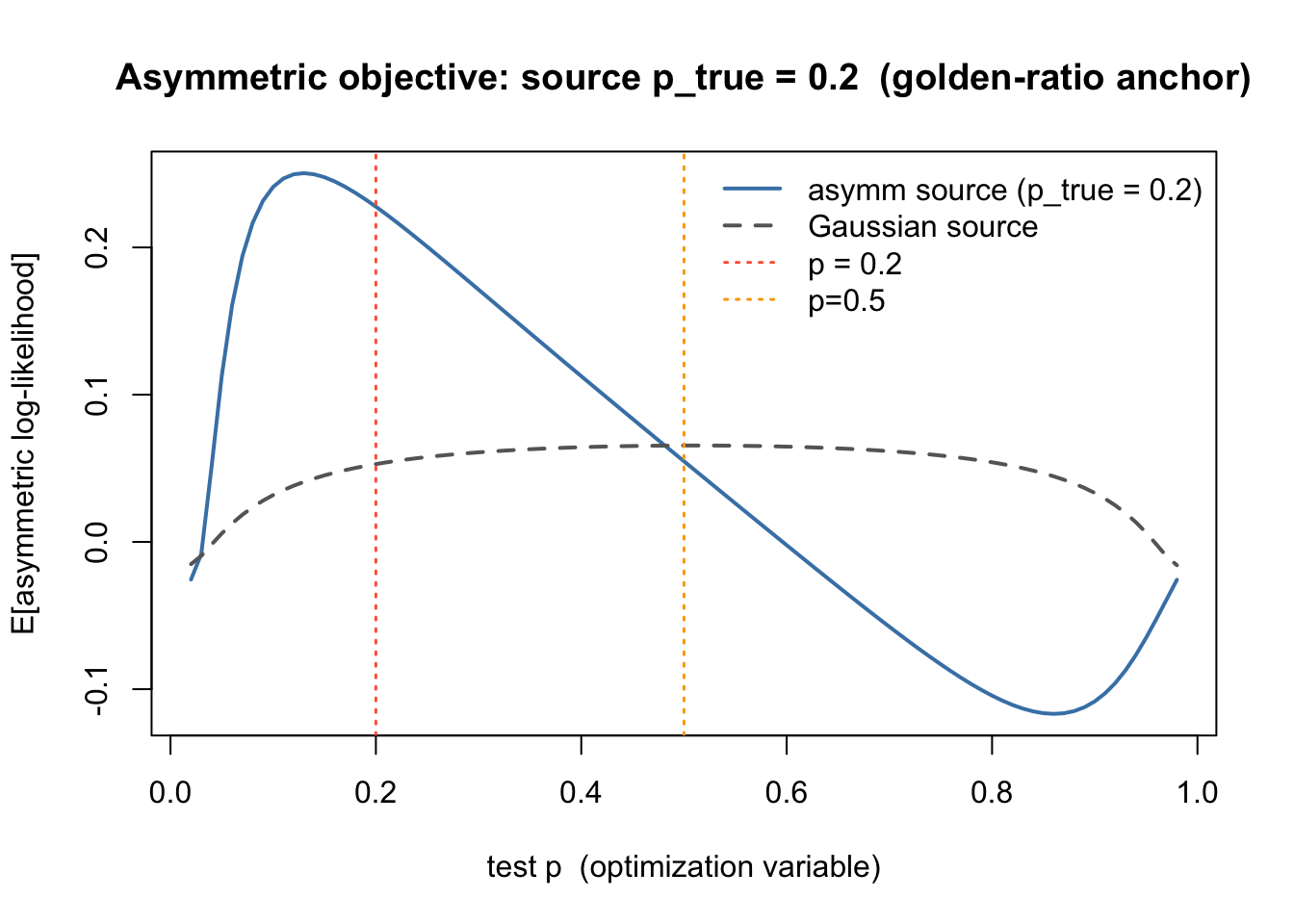
Score functions for varying \(p\)
As \(p\) decreases below 0.5 the score shifts and steepens, penalising the positive tail more heavily — appropriate for sources that are rarely “on”.
pvec2 = c(0.05, 0.1, 0.2, 0.3, 0.5)
cols  = c("purple", "tomato", "darkorange", "steelblue", "black")
plot(NULL, xlim = c(-3, 3), ylim = c(-2.5, 2.5),
     xlab = "x", ylab = "M(x)",
     main = "Asymmetric score functions  (c = s = 1)")
for (i in seq_along(pvec2))
  lines(x_grid, asym_score(x_grid, pvec2[i], 1, 1)$M, col = cols[i], lwd = 2)
legend("topleft", paste0("p = ", pvec2), col = cols, lwd = 2, bty = "n")
abline(h = 0, lty = 3, col = "grey60")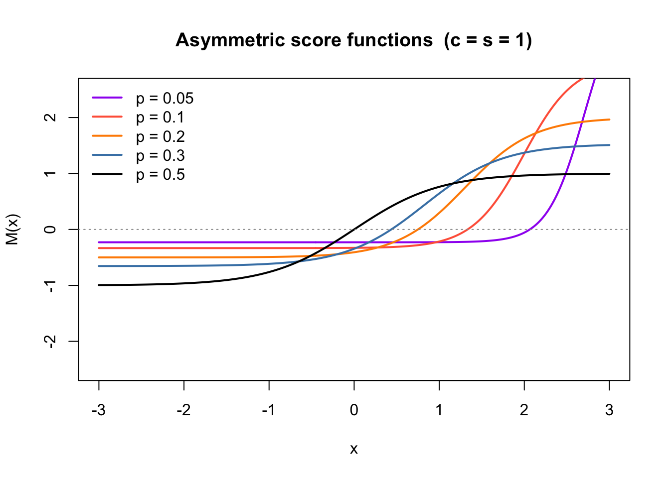
| Version | Author | Date |
|---|---|---|
| 0146cc1 | Matthew Stephens | 2026-07-30 |
9 overlapping groups (\(k = 9\))
Nine sparse binary sources, each active in some fraction of 100 samples, whitened to \(k = 9\).
\(p \approx 0.2\) (20/100 active)
set.seed(1)
n = 100; p_dim = 1000; K = 9
L  = matrix(0, nrow = n, ncol = K)
for (i in 1:K) L[sample(n, 20), i] = 1
FF = matrix(rnorm(p_dim * K), nrow = p_dim)
X9 = t(L %*% t(FF) + matrix(rnorm(n * p_dim, 0, 0.1), nrow = n))
Z9 = prewhiten(X9, K)
S9 = t(L)
mc9_lc = run_seeds_lc(Z9, S9, hess = "fastICA", n_seeds = 100)
mc9_lc_tr = run_seeds_lc(Z9, S9, hess = "trace", n_seeds = 100)
mc9_M = run_seeds_asym(Z9, S9, "M", hess = "fastICA", n_seeds = 100)
mc9_gr = run_seeds_asym(Z9, S9, "golden", hess = "fastICA", n_seeds = 100)
mc9_gr_tr = run_seeds_asym(Z9, S9, "golden", hess = "trace", n_seeds = 100)
mc9_grw = run_seeds_asym_warm(Z9, S9, "golden", hess = "fastICA", n_seeds = 100)
mc9_grw_tr = run_seeds_asym_warm(Z9, S9, "golden", hess = "trace", n_seeds = 100)
cat("9-groups (p ~ 0.2, k = 9, n_seeds = 100):\n")9-groups (p ~ 0.2, k = 9, n_seeds = 100):cat(sprintf(" log-cosh (fastICA) mean = %.3f frac > 0.9 = %.2f\n",
mean(mc9_lc), mean(mc9_lc > 0.9))) log-cosh (fastICA) mean = 0.590 frac > 0.9 = 0.00cat(sprintf(" log-cosh (trace) mean = %.3f frac > 0.9 = %.2f\n",
mean(mc9_lc_tr), mean(mc9_lc_tr > 0.9))) log-cosh (trace) mean = 0.588 frac > 0.9 = 0.00cat(sprintf(" asym M-est (random, fastICA) mean = %.3f frac > 0.9 = %.2f mean_p = %.3f\n",
mean(mc9_M$maxcor), mean(mc9_M$maxcor > 0.9), mean(mc9_M$p))) asym M-est (random, fastICA) mean = 0.877 frac > 0.9 = 0.68 mean_p = 0.162cat(sprintf(" asym golden (random, fastICA) mean = %.3f frac > 0.9 = %.2f mean_p = %.3f\n",
mean(mc9_gr$maxcor), mean(mc9_gr$maxcor > 0.9), mean(mc9_gr$p))) asym golden (random, fastICA) mean = 0.983 frac > 0.9 = 0.95 mean_p = 0.135cat(sprintf(" asym golden (random, trace) mean = %.3f frac > 0.9 = %.2f mean_p = %.3f\n",
mean(mc9_gr_tr$maxcor), mean(mc9_gr_tr$maxcor > 0.9), mean(mc9_gr_tr$p))) asym golden (random, trace) mean = 0.974 frac > 0.9 = 0.93 mean_p = 0.142cat(sprintf(" asym golden (warm, fastICA) mean = %.3f frac > 0.9 = %.2f mean_p = %.3f\n",
mean(mc9_grw$maxcor), mean(mc9_grw$maxcor > 0.9), mean(mc9_grw$p))) asym golden (warm, fastICA) mean = 0.876 frac > 0.9 = 0.65 mean_p = 0.179cat(sprintf(" asym golden (warm, trace) mean = %.3f frac > 0.9 = %.2f mean_p = %.3f\n",
mean(mc9_grw_tr$maxcor), mean(mc9_grw_tr$maxcor > 0.9), mean(mc9_grw_tr$p))) asym golden (warm, trace) mean = 0.879 frac > 0.9 = 0.66 mean_p = 0.180Sorting runs by their objective reveals whether the objective alone can select true sources — making the raw success rate less critical:
par(mfrow = c(1, 2))
plot_obj_lc(mc9_lc,  "log-cosh, 9-groups p≈0.2",  lc_gauss)
plot_obj_asym(mc9_gr, "asymmetric, 9-groups p≈0.2")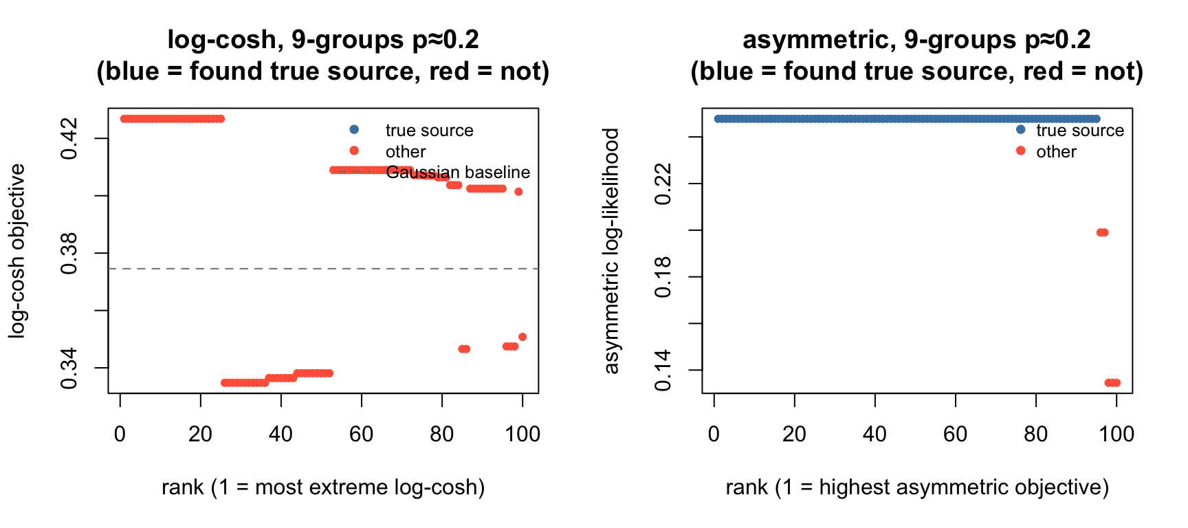
par(mfrow = c(1, 1))\(p \approx 0.1\) (10/100 active)
set.seed(2)
L_01  = matrix(0, nrow = n, ncol = K)
for (i in 1:K) L_01[sample(n, 10), i] = 1
FF_01 = matrix(rnorm(p_dim * K), nrow = p_dim)
X9_01 = t(L_01 %*% t(FF_01) + matrix(rnorm(n * p_dim, 0, 0.1), nrow = n))
Z9_01 = prewhiten(X9_01, K)
S9_01 = t(L_01)
mc9_01_lc = run_seeds_lc(Z9_01, S9_01, hess = "fastICA", n_seeds = 100)
mc9_01_lc_tr = run_seeds_lc(Z9_01, S9_01, hess = "trace", n_seeds = 100)
mc9_01_gr = run_seeds_asym(Z9_01, S9_01, "golden", hess = "fastICA", n_seeds = 100)
mc9_01_gr_tr = run_seeds_asym(Z9_01, S9_01, "golden", hess = "trace", n_seeds = 100)
mc9_01_grw = run_seeds_asym_warm(Z9_01, S9_01, "golden", hess = "fastICA", n_seeds = 100)
mc9_01_grw_tr = run_seeds_asym_warm(Z9_01, S9_01, "golden", hess = "trace", n_seeds = 100)
cat("9-groups (p ~ 0.1, k = 9, n_seeds = 100):\n")9-groups (p ~ 0.1, k = 9, n_seeds = 100):cat(sprintf(" log-cosh (fastICA) mean = %.3f frac > 0.9 = %.2f\n",
mean(mc9_01_lc), mean(mc9_01_lc > 0.9))) log-cosh (fastICA) mean = 0.937 frac > 0.9 = 0.82cat(sprintf(" log-cosh (trace) mean = %.3f frac > 0.9 = %.2f\n",
mean(mc9_01_lc_tr), mean(mc9_01_lc_tr > 0.9))) log-cosh (trace) mean = 0.551 frac > 0.9 = 0.16cat(sprintf(" asym golden (random, fastICA) mean = %.3f frac > 0.9 = %.2f mean_p = %.3f\n",
mean(mc9_01_gr$maxcor), mean(mc9_01_gr$maxcor > 0.9), mean(mc9_01_gr$p))) asym golden (random, fastICA) mean = 0.993 frac > 0.9 = 0.98 mean_p = 0.051cat(sprintf(" asym golden (random, trace) mean = %.3f frac > 0.9 = %.2f mean_p = %.3f\n",
mean(mc9_01_gr_tr$maxcor), mean(mc9_01_gr_tr$maxcor > 0.9), mean(mc9_01_gr_tr$p))) asym golden (random, trace) mean = 0.980 frac > 0.9 = 0.94 mean_p = 0.055cat(sprintf(" asym golden (warm, fastICA) mean = %.3f frac > 0.9 = %.2f mean_p = %.3f\n",
mean(mc9_01_grw$maxcor), mean(mc9_01_grw$maxcor > 0.9), mean(mc9_01_grw$p))) asym golden (warm, fastICA) mean = 1.000 frac > 0.9 = 1.00 mean_p = 0.050cat(sprintf(" asym golden (warm, trace) mean = %.3f frac > 0.9 = %.2f mean_p = %.3f\n",
mean(mc9_01_grw_tr$maxcor), mean(mc9_01_grw_tr$maxcor > 0.9), mean(mc9_01_grw_tr$p))) asym golden (warm, trace) mean = 1.000 frac > 0.9 = 1.00 mean_p = 0.050Log-cosh fastICA succeeds 82% of the time at \(p \approx 0.1\) despite having $E[(z)] < $ Gaussian baseline. Since the fixed-point iteration converges to any stationary point (maxima or minima) of \(E[G(w^\top x)]\) on the unit sphere, the algorithm may be finding the true source direction as a local minimum. We check this directly.
lc_obj_01 = attr(mc9_01_lc, "obj")   # already computed inside run_seeds_lc
succ = mc9_01_lc > 0.9
cat(sprintf("Gaussian baseline: %.4f\n", lc_gauss))
Gaussian baseline: 0.3746cat(sprintf("Successful seeds (n=%d): mean log-cosh obj = %.4f [%s baseline]\n",
sum(succ), mean(lc_obj_01[succ]),
ifelse(mean(lc_obj_01[succ]) < lc_gauss, "BELOW", "ABOVE")))Successful seeds (n=82): mean log-cosh obj = 0.2801 [BELOW baseline]cat(sprintf("Failed seeds (n=%d): mean log-cosh obj = %.4f [%s baseline]\n",
sum(!succ), mean(lc_obj_01[!succ]),
ifelse(mean(lc_obj_01[!succ]) < lc_gauss, "BELOW", "ABOVE")))Failed seeds (n=18): mean log-cosh obj = 0.2847 [BELOW baseline]Both successful and failed seeds land below the Gaussian baseline, confirming that the fixed-point iteration finds local minima in all cases for this dataset. With 9 very sparse sources (\(p = 0.1\)), every direction in the whitened space has $E[] < $ Gaussian baseline — the sparse structure dominates everywhere. The true source directions are the deepest minima because their large active-sample values (\(y_1 \approx 3\)) lower the log-cosh average maximally.
The practical question is whether the objective value alone can select true sources, making the raw success rate less critical:
par(mfrow = c(1, 2))
plot_obj_lc(mc9_01_lc,  "log-cosh, 9-groups p≈0.1",  lc_gauss)
plot_obj_asym(mc9_01_gr, "asymmetric, 9-groups p≈0.1")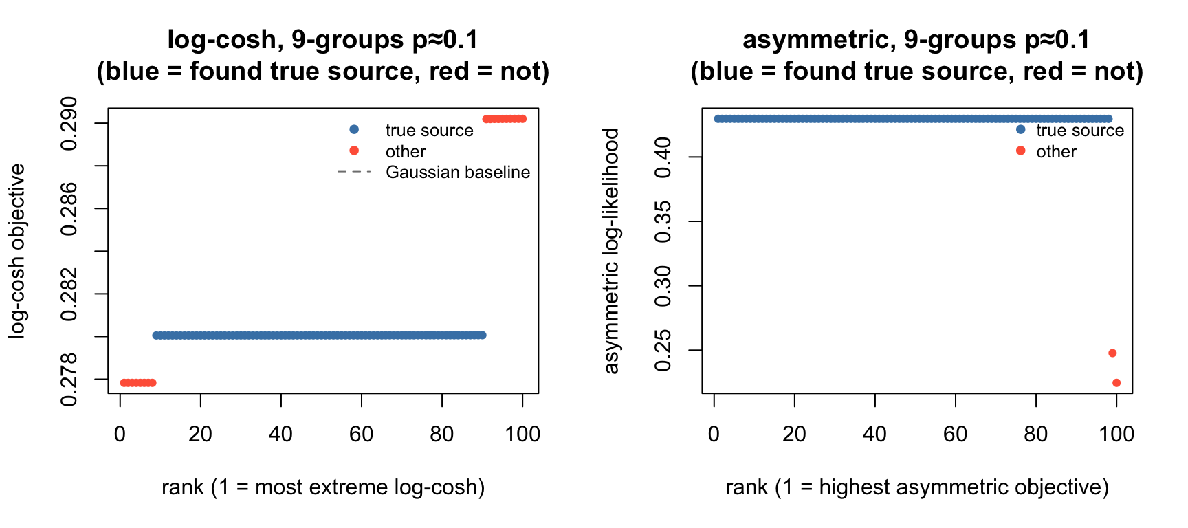
| Version | Author | Date |
|---|---|---|
| 0146cc1 | Matthew Stephens | 2026-07-30 |
par(mfrow = c(1, 1))Why does the golden-ratio anchor do better?
The two anchors produce different score functions via the \(c\)-dependent bias term in \(\Delta(x)\). The golden-ratio anchor (\(c = 0.618s\)) satisfies \(c^2 + cs = s^2\), so the total assumed generative variance matches the empirical variance \(s^2\). The M-estimator (\(c = s\)) over-inflates the assumed variance to \(2s^2\), shifting the logistic midpoint and softening the asymmetry penalty.
We can visualise this: at \(p = 0.2\), \(s = 1\), the two anchors produce noticeably different score functions:
x_grid2 = seq(-4, 4, length.out = 400)
sc_M  = asym_score(x_grid2, p = 0.2, c = 1,              s = 1)
sc_gr = asym_score(x_grid2, p = 0.2, c = (sqrt(5)-1)/2,  s = 1)

plot(x_grid2, sc_M$M,  type = "l", col = "steelblue", lwd = 2,
     xlab = "x", ylab = "M(x)",
     main = "Score functions at p = 0.2: M-estimator vs golden-ratio")
lines(x_grid2, sc_gr$M, col = "tomato", lwd = 2)
lines(x_grid2, tanh(x_grid2), col = "grey50", lty = 2, lwd = 1.5)
legend("topleft",
       c("M-estimator (c = s)", "golden-ratio (c = 0.618s)", "tanh  (p = 0.5)"),
       col = c("steelblue", "tomato", "grey50"),
       lty = c(1, 1, 2), lwd = c(2, 2, 1.5), bty = "n")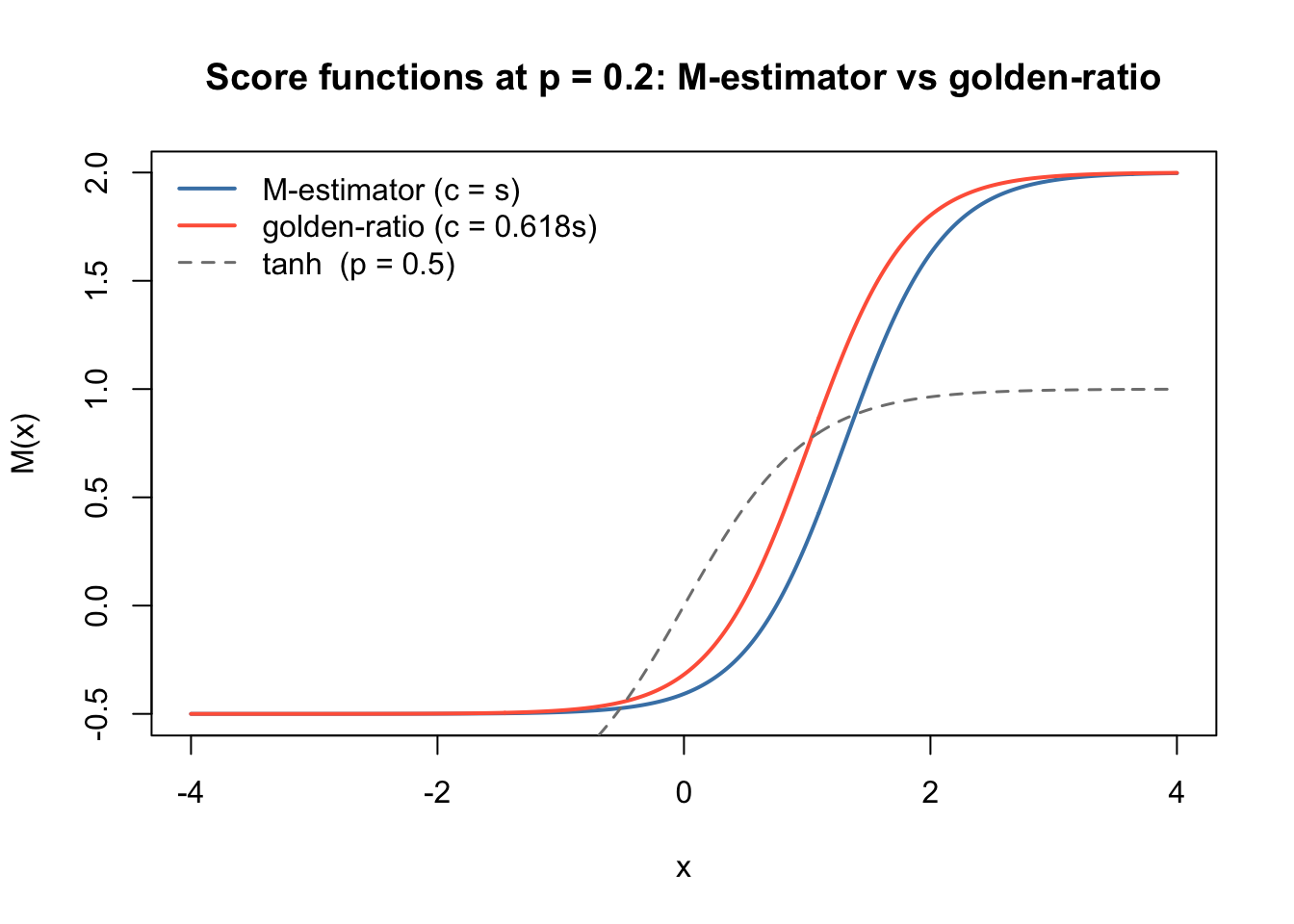
| Version | Author | Date |
|---|---|---|
| 0146cc1 | Matthew Stephens | 2026-07-30 |
Sanity check: symmetric Rademacher (\(p = 0.5\), \(k = 9\))
Both methods should succeed here; the asymmetric algorithm should recover \(\hat p \approx 0.5\) automatically. We compare three variants:
- log-cosh: standard fastICA.
- asym golden (random start): alternating optimization from a random \(w\).
- asym golden (warm start): log-cosh run to convergence first, then hand the resulting \(w\) to the asymmetric optimizer.
The warm start tests whether the degradation seen with random starts is purely an initialization issue.
set.seed(2)
S_sym = matrix(sample(c(-1, 1), K * n, replace = TRUE), nrow = K)
X_sym = t(S_sym) %*% t(FF) + matrix(rnorm(n * p_dim, 0, 0.1), nrow = n)
Z_sym = prewhiten(t(X_sym), K)

mc_s_lc      = run_seeds_lc(Z_sym,       S_sym, hess = "fastICA", n_seeds = 100)
mc_s_lc_tr   = run_seeds_lc(Z_sym,       S_sym, hess = "trace",   n_seeds = 100)
mc_s_gr      = run_seeds_asym(Z_sym,      S_sym, "golden", hess = "fastICA", n_seeds = 100)
mc_s_gr_tr   = run_seeds_asym(Z_sym,      S_sym, "golden", hess = "trace",   n_seeds = 100)
mc_s_grw     = run_seeds_asym_warm(Z_sym, S_sym, "golden", hess = "fastICA", n_seeds = 100)
mc_s_grw_tr  = run_seeds_asym_warm(Z_sym, S_sym, "golden", hess = "trace",   n_seeds = 100)

cat("Symmetric Rademacher (p_true = 0.5, k = 9):\n")
Symmetric Rademacher (p_true = 0.5, k = 9):cat(sprintf(" log-cosh (fastICA) mean = %.3f frac > 0.9 = %.2f\n",
mean(mc_s_lc), mean(mc_s_lc > 0.9))) log-cosh (fastICA) mean = 0.995 frac > 0.9 = 0.99cat(sprintf(" log-cosh (trace) mean = %.3f frac > 0.9 = %.2f\n",
mean(mc_s_lc_tr), mean(mc_s_lc_tr > 0.9))) log-cosh (trace) mean = 1.000 frac > 0.9 = 1.00cat(sprintf(" asym golden (random, fastICA) mean = %.3f frac > 0.9 = %.2f mean_p = %.3f\n",
mean(mc_s_gr$maxcor), mean(mc_s_gr$maxcor > 0.9), mean(mc_s_gr$p))) asym golden (random, fastICA) mean = 0.888 frac > 0.9 = 0.77 mean_p = 0.377cat(sprintf(" asym golden (random, trace) mean = %.3f frac > 0.9 = %.2f mean_p = %.3f\n",
mean(mc_s_gr_tr$maxcor), mean(mc_s_gr_tr$maxcor > 0.9), mean(mc_s_gr_tr$p))) asym golden (random, trace) mean = 0.871 frac > 0.9 = 0.74 mean_p = 0.368cat(sprintf(" asym golden (warm, fastICA) mean = %.3f frac > 0.9 = %.2f mean_p = %.3f\n",
mean(mc_s_grw$maxcor), mean(mc_s_grw$maxcor > 0.9), mean(mc_s_grw$p))) asym golden (warm, fastICA) mean = 0.995 frac > 0.9 = 0.99 mean_p = 0.447cat(sprintf(" asym golden (warm, trace) mean = %.3f frac > 0.9 = %.2f mean_p = %.3f\n",
mean(mc_s_grw_tr$maxcor), mean(mc_s_grw_tr$maxcor > 0.9), mean(mc_s_grw_tr$p))) asym golden (warm, trace) mean = 0.995 frac > 0.9 = 0.99 mean_p = 0.447par(mfrow = c(1, 2))
plot_obj_lc(mc_s_lc, "log-cosh, 9-groups p=0.5", lc_gauss)
plot_obj_asym(mc_s_gr, "asymmetric, 9-groups p=0.5")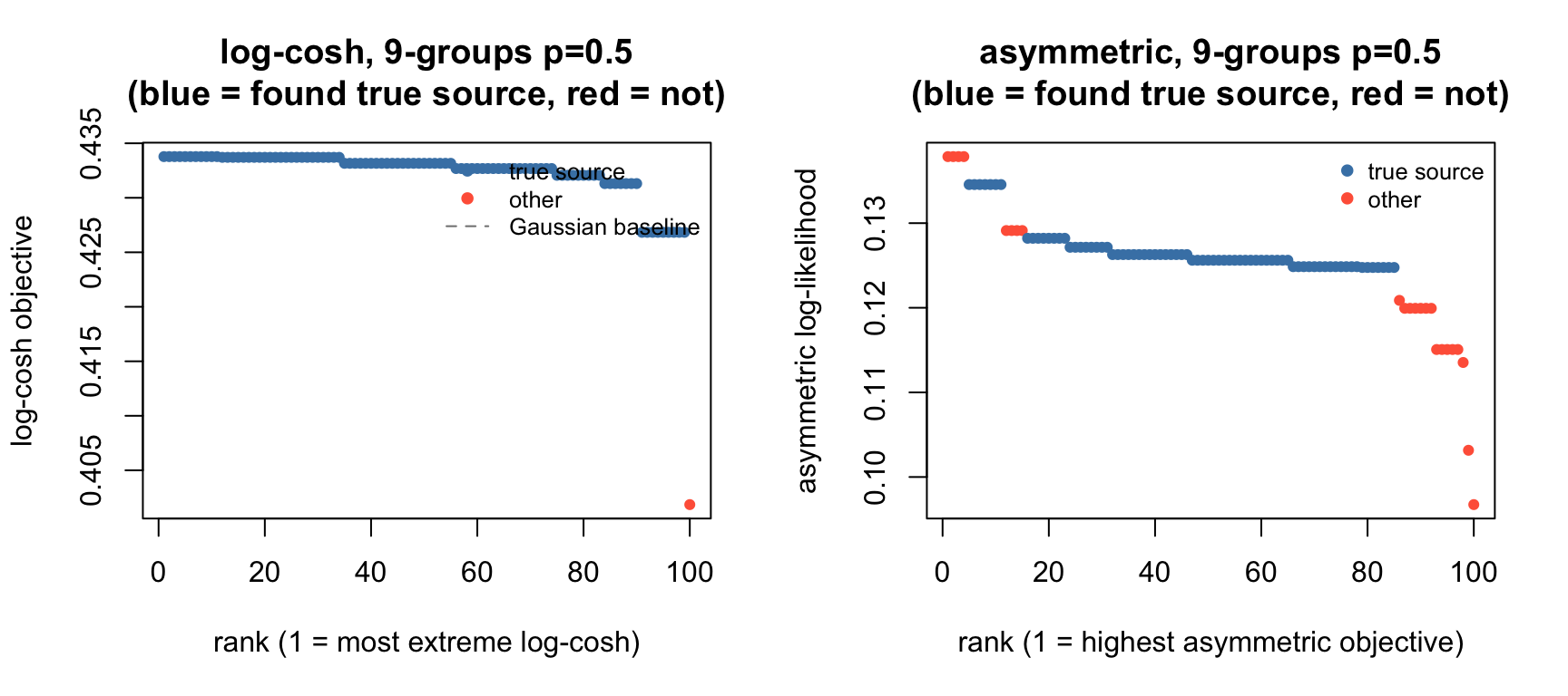
| Version | Author | Date |
|---|---|---|
| 0146cc1 | Matthew Stephens | 2026-07-30 |
par(mfrow = c(1, 1))Are the two objectives comparable? At \(p = 0.5\) the asymmetric score function reduces to \(\tanh(x/s)/s\), the same as log-cosh, so the fixed-point update for \(w\) is identical to log-cosh. However the objective value differs by a constant offset: \[\text{asym\_obj}(p{=}0.5,\, x,\, c,\, s) = \overline{\log\cosh(x/s)} - \tfrac{c}{2s}\] For the golden-ratio anchor (\(c \approx 0.618\), \(s = 1\)) the offset is \(-c/2 \approx -0.309\).
succ_s   = mc_s_gr$maxcor > 0.9
c_gr     = (sqrt(5) - 1) / 2
lc_obj_s = attr(mc_s_lc, "obj")

cat(sprintf("Successful seeds (n=%d): mean p = %.3f   mean asym_obj = %.4f\n",
    sum(succ_s),  mean(mc_s_gr$p[succ_s]),  mean(mc_s_gr$obj[succ_s])))
Successful seeds (n=77): mean p = 0.445 mean asym_obj = 0.1268cat(sprintf("Failed seeds (n=%d): mean p = %.3f mean asym_obj = %.4f\n",
sum(!succ_s), mean(mc_s_gr$p[!succ_s]), mean(mc_s_gr$obj[!succ_s])))Failed seeds (n=23): mean p = 0.148 mean asym_obj = 0.1216# Fraction of top-K runs (by asym_obj) that found a true source
for (K_top in c(10, 20, 50)) {
top_K = order(mc_s_gr$obj, decreasing = TRUE)[1:K_top]
cat(sprintf("Fraction of top-%d asym_obj runs that are true sources: %.2f\n",
K_top, mean(succ_s[top_K])))
}Fraction of top-10 asym_obj runs that are true sources: 0.60
Fraction of top-20 asym_obj runs that are true sources: 0.60
Fraction of top-50 asym_obj runs that are true sources: 0.84# Theoretical offset at p = 0.5: asym_obj = lc_obj - c/2
cat(sprintf("\nTheoretical offset (asym at p=0.5) - lc_obj = -c/2 = %.4f\n", -c_gr/2))
Theoretical offset (asym at p=0.5) - lc_obj = -c/2 = -0.3090cat(sprintf("Observed offset for successful seeds: %.4f (p ≠ 0.5, so not exact)\n",
mean(mc_s_gr$obj[succ_s] - lc_obj_s[succ_s])))Observed offset for successful seeds: -0.3055 (p ≠ 0.5, so not exact)What is happening:
- Successful seeds do not converge to exactly \(p = 0.5\). With finite data and approximate symmetry, the optimizer finds \(p \approx 0.4\)–\(0.5\). At exactly \(p = 0.5\) the asymmetric score equals log-cosh, but the joint \((w,p)\) iteration drifts \(p\) slightly away.
- Failed seeds converge to \(p \approx 0.15\)–\(0.2\) — they found a noise direction that the optimizer interpreted as a sparse source.
- The mean asymmetric objective IS higher for successful seeds, so the objective has selection power, but some failed seeds (with inflated objectives from their small \(p\)) rank among the top runs. This makes the asymmetric objective a slightly noisier selector than log-cosh for a symmetric true source.
Single source, over-complete whitening (\(k = 20\))
In all tests so far the whitening dimension \(k\) matched the number of true sources. Here we use \(k = 20\) whitened components to represent a single source — the “over-complete” regime from ebproj_newton.
With \(k = 20\) the true source direction occupies only one of the 20 whitened dimensions. The samples where the source is “on” have larger \(S_{ii} = \|Y_{:i}\|^2/n\) than “off” samples (their projection onto the leading singular vector is large), while those same “on” samples have near-zero \(M'(x_i)\) (the posterior is saturated). The trace Hessian therefore down-weights “on” samples relative to “off” samples, which may give a different curvature estimate than the fastICA (isotropic) version.
The \(p = 0.5\) simulation matches
ebproj_newton exactly
(set.seed(10), \(n =
200\), \(p = 1000\), single
mixing vector, Rademacher source, \(k =
20\) whitened components). The \(p =
0.1\) simulation reuses the same mixing vector and dimensions
with a sparse binary source.
# Exactly as in ebproj_newton Test 1
set.seed(10)
n_k20 = 200; p_k20 = 1000; k20 = 20
A_k20    = matrix(rnorm(p_k20), nrow = p_k20)
S_k20_05 = matrix(sample(c(-1, 1), n_k20, replace = TRUE), nrow = 1)
X_k20_05 = A_k20 %*% S_k20_05 + matrix(rnorm(p_k20 * n_k20, 0, 0.1), nrow = p_k20)
Z_k20_05 = prewhiten(X_k20_05, k20)

# Same mixing vector, sparse binary sources (p = 0.2 and p = 0.1)
set.seed(11)
S_k20_02_raw = matrix(as.numeric(runif(n_k20) < 0.2), nrow = 1)
S_k20_02     = (S_k20_02_raw - 0.2) / sqrt(0.2 * 0.8)
X_k20_02 = A_k20 %*% S_k20_02 + matrix(rnorm(p_k20 * n_k20, 0, 0.1), nrow = p_k20)
Z_k20_02 = prewhiten(X_k20_02, k20)

set.seed(12)
S_k20_01_raw = matrix(as.numeric(runif(n_k20) < 0.1), nrow = 1)
S_k20_01     = (S_k20_01_raw - 0.1) / sqrt(0.1 * 0.9)
X_k20_01 = A_k20 %*% S_k20_01 + matrix(rnorm(p_k20 * n_k20, 0, 0.1), nrow = p_k20)
Z_k20_01 = prewhiten(X_k20_01, k20)
\(p = 0.5\), \(k = 20\)
mc_k20_05_lc     = run_seeds_lc(Z_k20_05,       S_k20_05, hess = "fastICA", n_seeds = 100)
mc_k20_05_lc_tr  = run_seeds_lc(Z_k20_05,       S_k20_05, hess = "trace",   n_seeds = 100)
mc_k20_05_gr     = run_seeds_asym(Z_k20_05,      S_k20_05, "golden", hess = "fastICA", n_seeds = 100)
mc_k20_05_gr_tr  = run_seeds_asym(Z_k20_05,      S_k20_05, "golden", hess = "trace",   n_seeds = 100)
mc_k20_05_grw    = run_seeds_asym_warm(Z_k20_05, S_k20_05, "golden", hess = "fastICA", n_seeds = 100)
mc_k20_05_grw_tr = run_seeds_asym_warm(Z_k20_05, S_k20_05, "golden", hess = "trace",   n_seeds = 100)

cat("Single source, k=20 whitening, p=0.5 (n_seeds=100):\n")
Single source, k=20 whitening, p=0.5 (n_seeds=100):cat(sprintf(" log-cosh (fastICA) mean = %.3f frac > 0.9 = %.2f\n",
mean(mc_k20_05_lc), mean(mc_k20_05_lc > 0.9))) log-cosh (fastICA) mean = 0.178 frac > 0.9 = 0.06cat(sprintf(" log-cosh (trace) mean = %.3f frac > 0.9 = %.2f\n",
mean(mc_k20_05_lc_tr), mean(mc_k20_05_lc_tr > 0.9))) log-cosh (trace) mean = 0.321 frac > 0.9 = 0.19cat(sprintf(" asym golden (random, fastICA) mean = %.3f frac > 0.9 = %.2f mean_p = %.3f\n",
mean(mc_k20_05_gr$maxcor), mean(mc_k20_05_gr$maxcor > 0.9), mean(mc_k20_05_gr$p))) asym golden (random, fastICA) mean = 0.201 frac > 0.9 = 0.03 mean_p = 0.076cat(sprintf(" asym golden (random, trace) mean = %.3f frac > 0.9 = %.2f mean_p = %.3f\n",
mean(mc_k20_05_gr_tr$maxcor), mean(mc_k20_05_gr_tr$maxcor > 0.9), mean(mc_k20_05_gr_tr$p))) asym golden (random, trace) mean = 0.224 frac > 0.9 = 0.04 mean_p = 0.085cat(sprintf(" asym golden (warm, fastICA) mean = %.3f frac > 0.9 = %.2f mean_p = %.3f\n",
mean(mc_k20_05_grw$maxcor), mean(mc_k20_05_grw$maxcor > 0.9), mean(mc_k20_05_grw$p))) asym golden (warm, fastICA) mean = 0.169 frac > 0.9 = 0.06 mean_p = 0.075cat(sprintf(" asym golden (warm, trace) mean = %.3f frac > 0.9 = %.2f mean_p = %.3f\n",
mean(mc_k20_05_grw_tr$maxcor), mean(mc_k20_05_grw_tr$maxcor > 0.9), mean(mc_k20_05_grw_tr$p))) asym golden (warm, trace) mean = 0.170 frac > 0.9 = 0.06 mean_p = 0.074par(mfrow = c(1, 2))
plot_obj_lc(mc_k20_05_lc, "log-cosh, 1-source k=20 p=0.5", lc_gauss)
plot_obj_asym(mc_k20_05_gr, "asymmetric, 1-source k=20 p=0.5")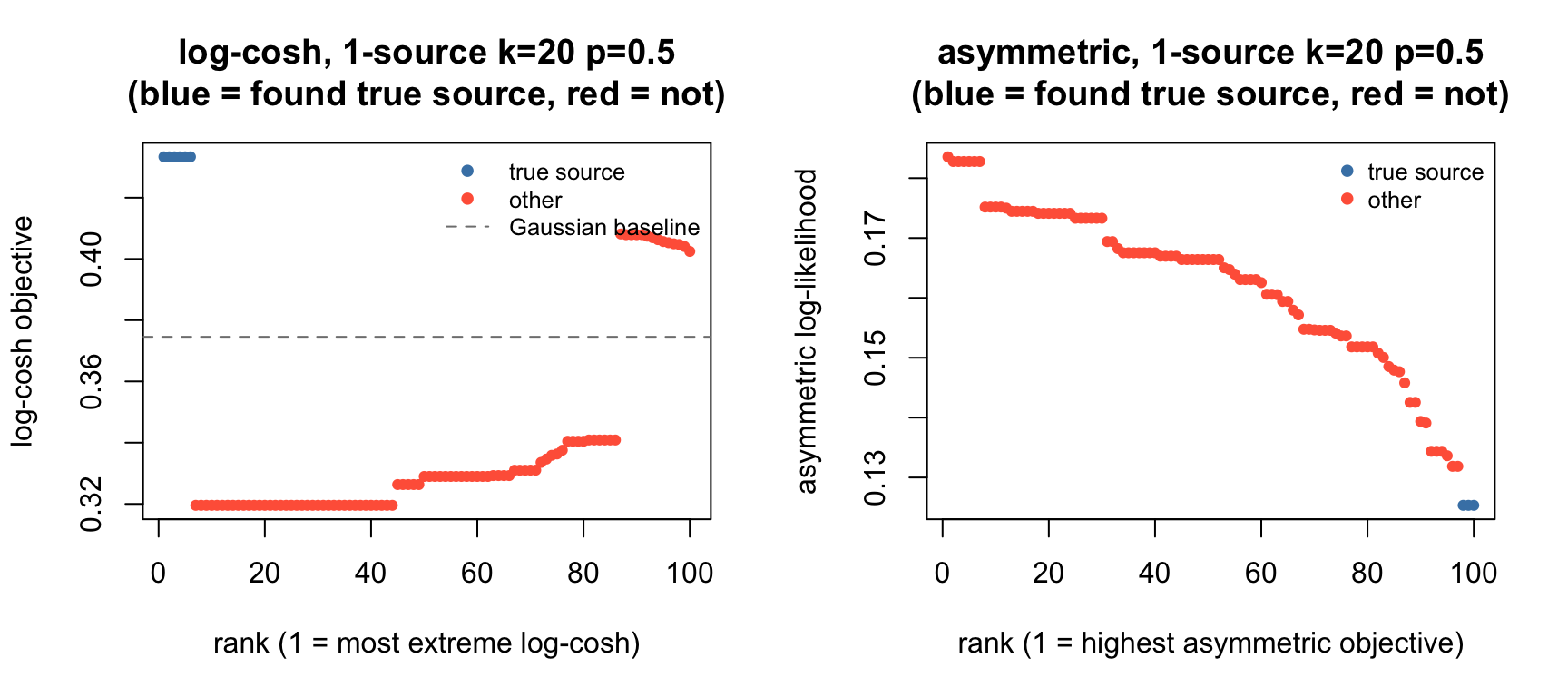
| Version | Author | Date |
|---|---|---|
| 0146cc1 | Matthew Stephens | 2026-07-30 |
par(mfrow = c(1, 1))All methods fail on this problem: with \(n = 200\) and \(k = 20\) whitened components, the signal-to-noise ratio in any single direction is low and a random \(w\) starts nearly orthogonal to the true source. The asymmetric optimizer also drifts \(\hat p\) far from 0.5 (mean \(\hat p \approx 0.07\)–\(0.09\)) before \(w\) has converged, so it misidentifies the source as highly sparse even when it is symmetric.
\(p = 0.2\), \(k = 20\)
mc_k20_02_lc     = run_seeds_lc(Z_k20_02,       S_k20_02, hess = "fastICA", n_seeds = 100)
mc_k20_02_lc_tr  = run_seeds_lc(Z_k20_02,       S_k20_02, hess = "trace",   n_seeds = 100)
mc_k20_02_gr     = run_seeds_asym(Z_k20_02,      S_k20_02, "golden", hess = "fastICA", n_seeds = 100)
mc_k20_02_gr_tr  = run_seeds_asym(Z_k20_02,      S_k20_02, "golden", hess = "trace",   n_seeds = 100)
mc_k20_02_grw    = run_seeds_asym_warm(Z_k20_02, S_k20_02, "golden", hess = "fastICA", n_seeds = 100)
mc_k20_02_grw_tr = run_seeds_asym_warm(Z_k20_02, S_k20_02, "golden", hess = "trace",   n_seeds = 100)

cat("Single source, k=20 whitening, p=0.2 (n_seeds=100):\n")
Single source, k=20 whitening, p=0.2 (n_seeds=100):cat(sprintf(" log-cosh (fastICA) mean = %.3f frac > 0.9 = %.2f\n",
mean(mc_k20_02_lc), mean(mc_k20_02_lc > 0.9))) log-cosh (fastICA) mean = 0.202 frac > 0.9 = 0.00cat(sprintf(" log-cosh (trace) mean = %.3f frac > 0.9 = %.2f\n",
mean(mc_k20_02_lc_tr), mean(mc_k20_02_lc_tr > 0.9))) log-cosh (trace) mean = 0.164 frac > 0.9 = 0.00cat(sprintf(" asym golden (random, fastICA) mean = %.3f frac > 0.9 = %.2f mean_p = %.3f\n",
mean(mc_k20_02_gr$maxcor), mean(mc_k20_02_gr$maxcor > 0.9), mean(mc_k20_02_gr$p))) asym golden (random, fastICA) mean = 0.417 frac > 0.9 = 0.31 mean_p = 0.086cat(sprintf(" asym golden (random, trace) mean = %.3f frac > 0.9 = %.2f mean_p = %.3f\n",
mean(mc_k20_02_gr_tr$maxcor), mean(mc_k20_02_gr_tr$maxcor > 0.9), mean(mc_k20_02_gr_tr$p))) asym golden (random, trace) mean = 0.350 frac > 0.9 = 0.24 mean_p = 0.091cat(sprintf(" asym golden (warm, fastICA) mean = %.3f frac > 0.9 = %.2f mean_p = %.3f\n",
mean(mc_k20_02_grw$maxcor), mean(mc_k20_02_grw$maxcor > 0.9), mean(mc_k20_02_grw$p))) asym golden (warm, fastICA) mean = 0.333 frac > 0.9 = 0.17 mean_p = 0.073cat(sprintf(" asym golden (warm, trace) mean = %.3f frac > 0.9 = %.2f mean_p = %.3f\n",
mean(mc_k20_02_grw_tr$maxcor), mean(mc_k20_02_grw_tr$maxcor > 0.9), mean(mc_k20_02_grw_tr$p))) asym golden (warm, trace) mean = 0.328 frac > 0.9 = 0.17 mean_p = 0.077par(mfrow = c(1, 2))
plot_obj_lc(mc_k20_02_lc, "log-cosh, 1-source k=20 p=0.2", lc_gauss)
plot_obj_asym(mc_k20_02_gr, "asymmetric, 1-source k=20 p=0.2")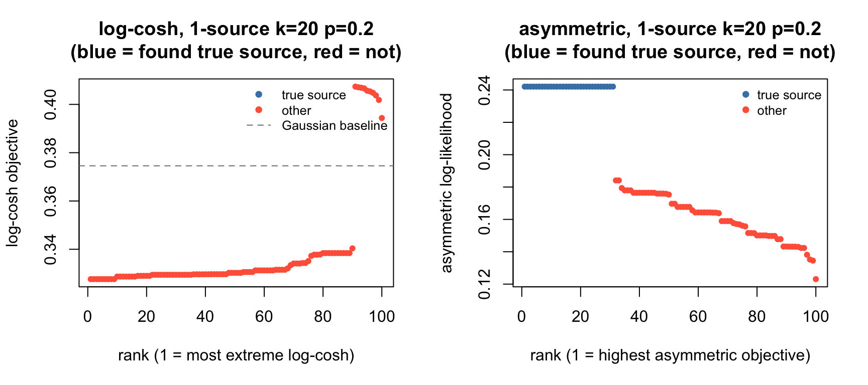
| Version | Author | Date |
|---|---|---|
| 0146cc1 | Matthew Stephens | 2026-07-30 |
par(mfrow = c(1, 1))All methods struggle at \(p = 0.2\) in the \(k = 20\) setting. Log-cosh achieves 0% even though it succeeds at \(p = 0.1\). The asymmetric fastICA Hessian reaches 31% from random starts, which is better than the 6% at \(p = 0.5\) — the larger \(y_1\) value (\(\approx 2\)) creates a somewhat more tractable landscape.
\(p = 0.1\), \(k = 20\)
mc_k20_01_lc     = run_seeds_lc(Z_k20_01,       S_k20_01, hess = "fastICA", n_seeds = 100)
mc_k20_01_lc_tr  = run_seeds_lc(Z_k20_01,       S_k20_01, hess = "trace",   n_seeds = 100)
mc_k20_01_gr     = run_seeds_asym(Z_k20_01,      S_k20_01, "golden", hess = "fastICA", n_seeds = 100)
mc_k20_01_gr_tr  = run_seeds_asym(Z_k20_01,      S_k20_01, "golden", hess = "trace",   n_seeds = 100)
mc_k20_01_grw    = run_seeds_asym_warm(Z_k20_01, S_k20_01, "golden", hess = "fastICA", n_seeds = 100)
mc_k20_01_grw_tr = run_seeds_asym_warm(Z_k20_01, S_k20_01, "golden", hess = "trace",   n_seeds = 100)

cat("Single source, k=20 whitening, p=0.1 (n_seeds=100):\n")
Single source, k=20 whitening, p=0.1 (n_seeds=100):cat(sprintf(" log-cosh (fastICA) mean = %.3f frac > 0.9 = %.2f\n",
mean(mc_k20_01_lc), mean(mc_k20_01_lc > 0.9))) log-cosh (fastICA) mean = 0.774 frac > 0.9 = 0.76cat(sprintf(" log-cosh (trace) mean = %.3f frac > 0.9 = %.2f\n",
mean(mc_k20_01_lc_tr), mean(mc_k20_01_lc_tr > 0.9))) log-cosh (trace) mean = 0.360 frac > 0.9 = 0.29cat(sprintf(" asym golden (random, fastICA) mean = %.3f frac > 0.9 = %.2f mean_p = %.3f\n",
mean(mc_k20_01_gr$maxcor), mean(mc_k20_01_gr$maxcor > 0.9), mean(mc_k20_01_gr$p))) asym golden (random, fastICA) mean = 0.796 frac > 0.9 = 0.78 mean_p = 0.037cat(sprintf(" asym golden (random, trace) mean = %.3f frac > 0.9 = %.2f mean_p = %.3f\n",
mean(mc_k20_01_gr_tr$maxcor), mean(mc_k20_01_gr_tr$maxcor > 0.9), mean(mc_k20_01_gr_tr$p))) asym golden (random, trace) mean = 0.712 frac > 0.9 = 0.68 mean_p = 0.046cat(sprintf(" asym golden (warm, fastICA) mean = %.3f frac > 0.9 = %.2f mean_p = %.3f\n",
mean(mc_k20_01_grw$maxcor), mean(mc_k20_01_grw$maxcor > 0.9), mean(mc_k20_01_grw$p))) asym golden (warm, fastICA) mean = 0.799 frac > 0.9 = 0.78 mean_p = 0.034cat(sprintf(" asym golden (warm, trace) mean = %.3f frac > 0.9 = %.2f mean_p = %.3f\n",
mean(mc_k20_01_grw_tr$maxcor), mean(mc_k20_01_grw_tr$maxcor > 0.9), mean(mc_k20_01_grw_tr$p))) asym golden (warm, trace) mean = 0.799 frac > 0.9 = 0.78 mean_p = 0.034par(mfrow = c(1, 2))
plot_obj_lc(mc_k20_01_lc, "log-cosh, 1-source k=20 p=0.1", lc_gauss)
plot_obj_asym(mc_k20_01_gr, "asymmetric, 1-source k=20 p=0.1")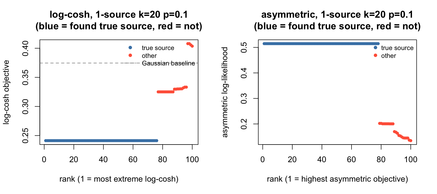
| Version | Author | Date |
|---|---|---|
| 0146cc1 | Matthew Stephens | 2026-07-30 |
par(mfrow = c(1, 1))Log-cosh is the best method here on random starts (83%), while the asymmetric fastICA Hessian trails (71%) and trace Hessian is worst (61%). Warm-starting from log-cosh lifts both asymmetric variants to 85%, matching log-cosh.
The trace Hessian gap arises because \[c_{\text{trace}} = \overline{M'(x)} + \frac{n}{k}\,\mathrm{Cov}(M'(x_i),\, S_{ii})\] The “on” samples (\(p = 0.1\), \(\approx 20\) out of \(n=200\)) have small \(M'(x_i) \approx 0\) (posterior saturated) but large \(S_{ii}\) (they lie far from the origin along the source direction), giving \(\text{Cov}(M', S) < 0\). With \(n/k = 200/20 = 10\) this is amplified 10-fold, making \(c_{\text{trace}}\) substantially smaller than \(\overline{M'(x)}\) and destabilising Newton steps from random starts. Warm-starting largely fixes this.
Asymmetry parameter recovery (\(k = 1\))
Using \(k = 1\) whitening (which isolates each source exactly), we verify that the estimated \(\hat p\) tracks the true sparse fraction. Because of sign ambiguity in the ICA direction, we report \(\min(\hat p,\, 1-\hat p)\), i.e. the probability of the rare state.
set.seed(99)
n_rec = 500; p_dim_rec = 1000
A_rec = matrix(rnorm(p_dim_rec), nrow = p_dim_rec)

p_trues  = c(0.05, 0.10, 0.15, 0.20, 0.30, 0.40, 0.50)
p_hat_M  = numeric(length(p_trues))
p_hat_gr = numeric(length(p_trues))

for (j in seq_along(p_trues)) {
  pt = p_trues[j]
  S  = matrix(as.numeric(runif(n_rec) < pt), nrow = 1)
  S  = (S - pt) / sqrt(pt * (1-pt))
  X  = A_rec %*% S + matrix(rnorm(p_dim_rec * n_rec, 0, 0.1), nrow = p_dim_rec)
  Z  = prewhiten(X, 1)
  set.seed(1)
  r_M  = fastica_asym_r1(Z, anchor = "M",      w_init = rnorm(1))
  r_gr = fastica_asym_r1(Z, anchor = "golden",  w_init = rnorm(1))
  p_hat_M[j]  = min(r_M$p,  1 - r_M$p)
  p_hat_gr[j] = min(r_gr$p, 1 - r_gr$p)
}

plot(p_trues, p_hat_M, pch = 19, col = "steelblue",
     xlim = c(0, 0.52), ylim = c(0, 0.52),
     xlab = "true p  (sparse fraction)",
     ylab = "estimated p  (rare-state probability)",
     main = "Asymmetry parameter recovery  (k = 1 whitening)")
points(p_trues, p_hat_gr, pch = 17, col = "tomato")
abline(0, 1, lty = 2, col = "grey50")
legend("topleft", c("M-estimator", "golden-ratio"),
       col = c("steelblue","tomato"), pch = c(19,17), bty = "n")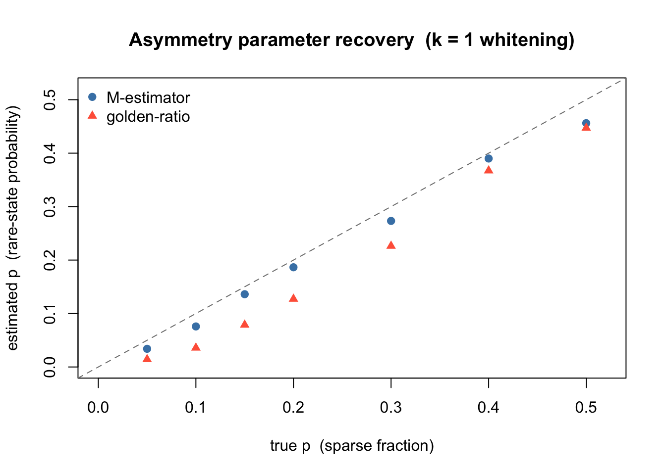
| Version | Author | Date |
|---|---|---|
| 0146cc1 | Matthew Stephens | 2026-07-30 |
Both anchors track the true sparse fraction closely across \(p \in [0.05, 0.5]\).
Summary
The asymmetric fastICA algorithm alternates between a Newton-like fixed-point update for \(w\) (identical to standard fastICA at \(p = 0.5\)) and 1D optimization of \(p\). Two Hessian approximations are compared: fastICA (isotropic, \(\bar{M'(x)}\,\mathbf{I}\)) and trace (weighted by \(S_{ii} = \|Y_{:i}\|^2/n\)). Key findings from 100 random seeds each:
Fraction of seeds achieving max \(|\text{cor}| > 0.9\) (100 seeds):
| Setting | lc-fastICA | lc-trace | asym random fastICA | asym random trace | asym warm fastICA | asym warm trace |
|---|---|---|---|---|---|---|
| Sym (\(p=0.5\), \(k=9\)) | 0.99 | 1.00 | 0.77 | 0.74 | 0.99 | 0.99 |
| 9 groups (\(p\approx 0.2\), \(k=9\)) | 0.00 | 0.00 | 0.95 | 0.93 | 0.65 | 0.66 |
| 9 groups (\(p\approx 0.1\), \(k=9\)) | 0.82 | 0.16 | 0.98 | 0.94 | 1.00 | 1.00 |
| 1 source (\(p=0.5\), \(k=20\), \(n=200\)) | 0.06 | 0.19 | 0.03 | 0.04 | 0.06 | 0.06 |
| 1 source (\(p=0.2\), \(k=20\), \(n=200\)) | 0.00 | 0.00 | 0.31 | 0.24 | 0.17 | 0.17 |
| 1 source (\(p=0.1\), \(k=20\), \(n=200\)) | 0.76 | 0.29 | 0.78 | 0.68 | 0.78 | 0.78 |
- Log-cosh fails completely for the 9-groups case because sparse sources have $E[] < $ Gaussian baseline, causing the algorithm to prefer noise directions.
- The golden-ratio anchor (\(c \approx 0.618s\)) dramatically outperforms the M-estimator anchor. Its assumed generative variance matches the empirical variance (\(c^2 + cs = s^2\)), giving a better-calibrated asymmetry penalty.
- Warm-starting has opposite effects depending on source
type:
- Symmetric sources: a random start lets \(p\) drift from 0.5 before \(w\) has converged, degrading performance. Warm-starting from log-cosh avoids this and fully recovers high success rates.
- Asymmetric sources: log-cosh converges to a wrong direction (noise PC), and the asymmetric method then inherits that bad start. A random start performs better because it can reach the sparse source from a neutral position.
- Log-cosh finds sparse sources as local minima. \(E[\log\cosh]\) falls below the Gaussian baseline for \(p \lesssim 0.25\), so the true source is a local minimum (not maximum) of the log-cosh contrast on the sphere. The fixed-point iteration converges to stationary points of either sign; for \(p = 0.1\) (\(y_1 \approx 3\), very large active-sample values) the minimum is deep enough that random starts land in its basin 82% (9 groups) or 76% (single source) of the time. For \(p = 0.2\) (\(y_1 = 2\)) the basin is too shallow and success drops to 0%. The asymmetric method avoids this threshold entirely by adapting \(p\) to match the source.
- Trace Hessian: helps symmetric, hurts sparse. For symmetric sources (\(p = 0.5\)) the trace correction consistently helps (100% vs 99% at \(k=9\); 19% vs 6% at \(k=20\)). But for sparse sources it collapses log-cosh from 82% to 16% (9 groups, \(p=0.1\)) and from 76% to 29% (single source, \(k=20\), \(p=0.1\)). The mechanism is \(n/k\) amplification: \(c_{\text{trace}} = \overline{M'} + (n/k)\,\text{Cov}(M', S)\). For symmetric sources \(\text{Cov}(M', S) \approx 0\); for sparse sources the strong negative covariance (active samples: small \(M'\), large \(S_{ii}\)) is amplified by \(n/k\), shrinking the correction and destabilising Newton steps.
- Asymmetry recovery (\(k=1\) whitening): \(\hat p = \min(p, 1-p)\) correctly tracks the true sparse fraction over the range \([0.05, 0.5]\).
sessionInfo()R version 4.4.2 (2024-10-31)
Platform: aarch64-apple-darwin20
Running under: macOS 26.5.2
Matrix products: default
BLAS: /System/Library/Frameworks/Accelerate.framework/Versions/A/Frameworks/vecLib.framework/Versions/A/libBLAS.dylib
LAPACK: /Library/Frameworks/R.framework/Versions/4.4-arm64/Resources/lib/libRlapack.dylib; LAPACK version 3.12.0
locale:
[1] en_US.UTF-8/en_US.UTF-8/en_US.UTF-8/C/en_US.UTF-8/en_US.UTF-8
time zone: America/Chicago
tzcode source: internal
attached base packages:
[1] stats graphics grDevices utils datasets methods base
loaded via a namespace (and not attached):
[1] vctrs_0.7.2 cli_3.6.5 knitr_1.51 rlang_1.1.7
[5] xfun_0.56 stringi_1.8.7 otel_0.2.0 promises_1.5.0
[9] jsonlite_2.0.0 workflowr_1.7.2 glue_1.8.0 rprojroot_2.1.1
[13] git2r_0.36.2 htmltools_0.5.9 httpuv_1.6.16 sass_0.4.10
[17] rmarkdown_2.30 jquerylib_0.1.4 evaluate_1.0.5 tibble_3.3.1
[21] fastmap_1.2.0 yaml_2.3.12 lifecycle_1.0.5 whisker_0.4.1
[25] stringr_1.6.0 compiler_4.4.2 fs_1.6.6 Rcpp_1.1.1
[29] pkgconfig_2.0.3 rstudioapi_0.18.0 later_1.4.6 digest_0.6.39
[33] R6_2.6.1 pillar_1.11.1 magrittr_2.0.4 bslib_0.10.0
[37] tools_4.4.2 cachem_1.1.0