FastICA with Tilted Log-Cosh
Matthew Stephens, with use of Gemini/Claude
2026-07-07
Last updated: 2026-08-21
Checks: 7 0
Knit directory: misc/analysis/
This reproducible R Markdown analysis was created with workflowr (version 1.7.2). The Checks tab describes the reproducibility checks that were applied when the results were created. The Past versions tab lists the development history.
Great! Since the R Markdown file has been committed to the Git repository, you know the exact version of the code that produced these results.
Great job! The global environment was empty. Objects defined in the global environment can affect the analysis in your R Markdown file in unknown ways. For reproduciblity it’s best to always run the code in an empty environment.
The command set.seed(1) was run prior to running the
code in the R Markdown file. Setting a seed ensures that any results
that rely on randomness, e.g. subsampling or permutations, are
reproducible.
Great job! Recording the operating system, R version, and package versions is critical for reproducibility.
Nice! There were no cached chunks for this analysis, so you can be confident that you successfully produced the results during this run.
Great job! Using relative paths to the files within your workflowr project makes it easier to run your code on other machines.
Great! You are using Git for version control. Tracking code development and connecting the code version to the results is critical for reproducibility.
The results in this page were generated with repository version 640bddd. See the Past versions tab to see a history of the changes made to the R Markdown and HTML files.
Note that you need to be careful to ensure that all relevant files for
the analysis have been committed to Git prior to generating the results
(you can use wflow_publish or
wflow_git_commit). workflowr only checks the R Markdown
file, but you know if there are other scripts or data files that it
depends on. Below is the status of the Git repository when the results
were generated:
Ignored files:
    Ignored:    .DS_Store
    Ignored:    .Rhistory
    Ignored:    .Rproj.user/
    Ignored:    .claude/
    Ignored:    GSE87571/
    Ignored:    analysis/.RData
    Ignored:    analysis/.Rhistory
    Ignored:    analysis/ALStruct_cache/
    Ignored:    analysis/binary_quad_comparison_cache/
    Ignored:    analysis/ebproj_01.html
    Ignored:    analysis/gset_G63_cache/
    Ignored:    data/.Rhistory
    Ignored:    data/methylation-data-for-matthew.rds
    Ignored:    data/pbmc/
    Ignored:    data/pbmc_purified.RData

Untracked files:
    Untracked:  .dropbox
    Untracked:  GSE41037/
    Untracked:  Icon
    Untracked:  Rplots.pdf
    Untracked:  analysis/GHstan.Rmd
    Untracked:  analysis/GTEX-cogaps.Rmd
    Untracked:  analysis/PACS.Rmd
    Untracked:  analysis/Rplot.png
    Untracked:  analysis/SPCAvRP.rmd
    Untracked:  analysis/abf_comparisons.Rmd
    Untracked:  analysis/admm_02.Rmd
    Untracked:  analysis/admm_03.Rmd
    Untracked:  analysis/binary_quad_comparison.Rmd
    Untracked:  analysis/bispca.Rmd
    Untracked:  analysis/cache/
    Untracked:  analysis/cholesky.Rmd
    Untracked:  analysis/compare-transformed-models.Rmd
    Untracked:  analysis/cormotif.Rmd
    Untracked:  analysis/cp_ash.Rmd
    Untracked:  analysis/eQTL.perm.rand.pdf
    Untracked:  analysis/eb_power2.Rmd
    Untracked:  analysis/eb_prepilot.Rmd
    Untracked:  analysis/eb_var.Rmd
    Untracked:  analysis/ebpmf1.Rmd
    Untracked:  analysis/ebpmf_sla_text.Rmd
    Untracked:  analysis/ebproj_01.Rmd
    Untracked:  analysis/ebproj_newton.Rmd
    Untracked:  analysis/ebspca_sims.Rmd
    Untracked:  analysis/explore_psvd.Rmd
    Untracked:  analysis/fa_check_identify.Rmd
    Untracked:  analysis/fa_iterative.Rmd
    Untracked:  analysis/fastica_heated.Rmd
    Untracked:  analysis/fastica_unwhitened.Rmd
    Untracked:  analysis/flash_cov_overlapping_groups_init.Rmd
    Untracked:  analysis/flash_test_tree.Rmd
    Untracked:  analysis/flashier_newgroups.Rmd
    Untracked:  analysis/flashier_nmf_triples.Rmd
    Untracked:  analysis/flashier_pbmc.Rmd
    Untracked:  analysis/flashier_snn_shifted_prior.Rmd
    Untracked:  analysis/greedy_ebpmf_exploration_00.Rmd
    Untracked:  analysis/gset_G63.Rmd
    Untracked:  analysis/ieQTL.perm.rand.pdf
    Untracked:  analysis/lasso_em_03.Rmd
    Untracked:  analysis/m6amash.Rmd
    Untracked:  analysis/mash_bhat_z.Rmd
    Untracked:  analysis/mash_ieqtl_permutations.Rmd
    Untracked:  analysis/matrix_beta.Rmd
    Untracked:  analysis/meth_flash_01.Rmd
    Untracked:  analysis/methylation_example.Rmd
    Untracked:  analysis/mixsqp.Rmd
    Untracked:  analysis/mr.ash_lasso_init.Rmd
    Untracked:  analysis/mr.mash.test.Rmd
    Untracked:  analysis/mr_ash_modular.Rmd
    Untracked:  analysis/mr_ash_parameterization.Rmd
    Untracked:  analysis/mr_ash_ridge.Rmd
    Untracked:  analysis/mv_gaussian_message_passing.Rmd
    Untracked:  analysis/nejm.Rmd
    Untracked:  analysis/nmf_bg.Rmd
    Untracked:  analysis/nonneg_underapprox.Rmd
    Untracked:  analysis/normal_conditional_on_r2.Rmd
    Untracked:  analysis/normalize.Rmd
    Untracked:  analysis/pbmc.Rmd
    Untracked:  analysis/pca_binary_weighted.Rmd
    Untracked:  analysis/pca_l1.Rmd
    Untracked:  analysis/poisson_nmf_approx.Rmd
    Untracked:  analysis/poisson_shrink.Rmd
    Untracked:  analysis/poisson_transform.Rmd
    Untracked:  analysis/qrnotes.txt
    Untracked:  analysis/ridge_iterative_02.Rmd
    Untracked:  analysis/ridge_iterative_splitting.Rmd
    Untracked:  analysis/samps/
    Untracked:  analysis/sc_bimodal.Rmd
    Untracked:  analysis/shrinkage_comparisons_changepoints.Rmd
    Untracked:  analysis/susie_cov.Rmd
    Untracked:  analysis/susie_en.Rmd
    Untracked:  analysis/susie_z_investigate.Rmd
    Untracked:  analysis/svd-timing.Rmd
    Untracked:  analysis/temp.RDS
    Untracked:  analysis/temp.Rmd
    Untracked:  analysis/test-figure/
    Untracked:  analysis/test.Rmd
    Untracked:  analysis/test.Rpres
    Untracked:  analysis/test.md
    Untracked:  analysis/test_qr.R
    Untracked:  analysis/test_sparse.Rmd
    Untracked:  analysis/tree_dist_top_eigenvector.Rmd
    Untracked:  analysis/z.txt
    Untracked:  code/coordinate_descent_symNMF.R
    Untracked:  code/multivariate_testfuncs.R
    Untracked:  code/rqb.hacked.R
    Untracked:  data/4matthew/
    Untracked:  data/4matthew2/
    Untracked:  data/E-MTAB-2805.processed.1/
    Untracked:  data/ENSG00000156738.Sim_Y2.RDS
    Untracked:  data/G63
    Untracked:  data/GDS5363_full.soft.gz
    Untracked:  data/GSE41265_allGenesTPM.txt
    Untracked:  data/Muscle_Skeletal.ACTN3.pm1Mb.RDS
    Untracked:  data/P.rds
    Untracked:  data/Thyroid.FMO2.pm1Mb.RDS
    Untracked:  data/bmass.HaemgenRBC2016.MAF01.Vs2.MergedDataSources.200kRanSubset.ChrBPMAFMarkerZScores.vs1.txt.gz
    Untracked:  data/bmass.HaemgenRBC2016.Vs2.NewSNPs.ZScores.hclust.vs1.txt
    Untracked:  data/bmass.HaemgenRBC2016.Vs2.PreviousSNPs.ZScores.hclust.vs1.txt
    Untracked:  data/eb_prepilot/
    Untracked:  data/finemap_data/fmo2.sim/b.txt
    Untracked:  data/finemap_data/fmo2.sim/dap_out.txt
    Untracked:  data/finemap_data/fmo2.sim/dap_out2.txt
    Untracked:  data/finemap_data/fmo2.sim/dap_out2_snp.txt
    Untracked:  data/finemap_data/fmo2.sim/dap_out_snp.txt
    Untracked:  data/finemap_data/fmo2.sim/data
    Untracked:  data/finemap_data/fmo2.sim/fmo2.sim.config
    Untracked:  data/finemap_data/fmo2.sim/fmo2.sim.k
    Untracked:  data/finemap_data/fmo2.sim/fmo2.sim.k4.config
    Untracked:  data/finemap_data/fmo2.sim/fmo2.sim.k4.snp
    Untracked:  data/finemap_data/fmo2.sim/fmo2.sim.ld
    Untracked:  data/finemap_data/fmo2.sim/fmo2.sim.snp
    Untracked:  data/finemap_data/fmo2.sim/fmo2.sim.z
    Untracked:  data/finemap_data/fmo2.sim/pos.txt
    Untracked:  data/logm.csv
    Untracked:  data/m.cd.RDS
    Untracked:  data/m.cdu.old.RDS
    Untracked:  data/m.new.cd.RDS
    Untracked:  data/m.old.cd.RDS
    Untracked:  data/mainbib.bib.old
    Untracked:  data/mat.csv
    Untracked:  data/mat.txt
    Untracked:  data/mat_new.csv
    Untracked:  data/matrix_lik.rds
    Untracked:  data/paintor_data/
    Untracked:  data/running_data_chris.csv
    Untracked:  data/running_data_matthew.csv
    Untracked:  data/temp.txt
    Untracked:  data/y.txt
    Untracked:  data/y_f.txt
    Untracked:  data/zscore_jointLCLs_m6AQTLs_susie_eQTLpruned.rds
    Untracked:  data/zscore_jointLCLs_random.rds
    Untracked:  explore_udi.R
    Untracked:  output/fit.k10.rds
    Untracked:  output/fit.nn.pbmc.purified.rds
    Untracked:  output/fit.nn.rds
    Untracked:  output/fit.nn.s.001.rds
    Untracked:  output/fit.nn.s.01.rds
    Untracked:  output/fit.nn.s.1.rds
    Untracked:  output/fit.nn.s.10.rds
    Untracked:  output/fit.snn.s.001.rds
    Untracked:  output/fit.snn.s.01.nninit.rds
    Untracked:  output/fit.snn.s.01.rds
    Untracked:  output/fit.varbvs.RDS
    Untracked:  output/fit2.nn.pbmc.purified.rds
    Untracked:  output/glmnet.fit.RDS
    Untracked:  output/snn07.txt
    Untracked:  output/snn34.txt
    Untracked:  output/test.bv.txt
    Untracked:  output/test.gamma.txt
    Untracked:  output/test.hyp.txt
    Untracked:  output/test.log.txt
    Untracked:  output/test.param.txt
    Untracked:  output/test2.bv.txt
    Untracked:  output/test2.gamma.txt
    Untracked:  output/test2.hyp.txt
    Untracked:  output/test2.log.txt
    Untracked:  output/test2.param.txt
    Untracked:  output/test3.bv.txt
    Untracked:  output/test3.gamma.txt
    Untracked:  output/test3.hyp.txt
    Untracked:  output/test3.log.txt
    Untracked:  output/test3.param.txt
    Untracked:  output/test4.bv.txt
    Untracked:  output/test4.gamma.txt
    Untracked:  output/test4.hyp.txt
    Untracked:  output/test4.log.txt
    Untracked:  output/test4.param.txt
    Untracked:  output/test5.bv.txt
    Untracked:  output/test5.gamma.txt
    Untracked:  output/test5.hyp.txt
    Untracked:  output/test5.log.txt
    Untracked:  output/test5.param.txt

Unstaged changes:
    Modified:   .gitignore
    Modified:   analysis/eb_snmu.Rmd
    Modified:   analysis/ebnm_binormal.Rmd
    Modified:   analysis/ebpower.Rmd
    Modified:   analysis/fastica_asymmetric_03.Rmd
    Modified:   analysis/fastica_bm_spd.Rmd
    Modified:   analysis/flashier_log1p.Rmd
    Modified:   analysis/flashier_sla_text.Rmd
    Modified:   analysis/logistic_z_scores.Rmd
    Modified:   analysis/mr_ash_pen.Rmd
    Modified:   analysis/nmu_em.Rmd
    Modified:   analysis/susie_flash.Rmd
    Modified:   analysis/tap_free_energy.Rmd
    Modified:   misc.Rproj
Note that any generated files, e.g. HTML, png, CSS, etc., are not included in this status report because it is ok for generated content to have uncommitted changes.
These are the previous versions of the repository in which changes were
made to the R Markdown (analysis/fastica_skew.Rmd) and HTML
(docs/fastica_skew.html) files. If you’ve configured a
remote Git repository (see ?wflow_git_remote), click on the
hyperlinks in the table below to view the files as they were in that
past version.
| File | Version | Author | Date | Message |
|---|---|---|---|---|
| Rmd | 640bddd | Matthew Stephens | 2026-08-21 | workflowr::wflow_publish("fastica_skew.Rmd") |
| html | e64a684 | Matthew Stephens | 2026-07-16 | Build site. |
| Rmd | cf3bf2f | Matthew Stephens | 2026-07-16 | Add noise to tests, 9-component plots |
| html | 7da05b8 | Matthew Stephens | 2026-07-16 | Build site. |
| Rmd | 159d466 | Matthew Stephens | 2026-07-16 | Add tilted log-cosh FastICA analysis |
Introduction
This implements and tests two asymmetric constrast functions for fastICA: the “Tilted Log-Cosh” (TLC) contrast function and one based on \(G(z) = \log(\Phi(\alpha z))\) where \(\Phi\) is the Cumulative Distribution Function (CDF) of the standard normal distribution, and \(\alpha\) is a fixed scalar (e.g., \(\alpha = 2\)). Both functions came up in conversations with Gemini.
The motivation for this is that the standard log-cosh contrast fails to detect highly skewed (sparse) binary sources because its expectation falls below the Gaussian baseline as \(p \to 0\) or \(p \to 1\). The tilted log-cosh version adds a \(\lambda z|z|\) term:
\[G(z) = \log(\cosh(z)) + \lambda z|z|\]
with derivatives: \[g(z) = \tanh(z) + 2\lambda|z|, \quad g'(z) = 1 - \tanh^2(z) + 2\lambda \text{sign}(z)\]
The odd term \(z|z|\) has expectation \(2p-1\) for a standardized binary source, so the tilted objective monotonically increases as \(p \to 1\), unlike log-cosh which peaks at \(p=0.5\).
Implementation
# Standard log-cosh FastICA (single component, rank-1 update)
fastica_r1update = function(X, w) {
  w = w / sqrt(sum(w^2))
  P = t(X) %*% w
  G  = tanh(P)
  G2 = 1 - tanh(P)^2
  w  = X %*% G - mean(G2) * ncol(X) * w
  w / sqrt(sum(w^2))
}

compute_objective = function(X, w) {
  P = t(X) %*% w
  mean(log(cosh(P)))
}

# Tilted log-cosh FastICA (single component)
fastica_r1update_tlc = function(X, w, lambda = 1) {
  w = w / sqrt(sum(w^2))
  P = t(X) %*% w
  G  = tanh(P) + 2 * lambda * abs(P)
  G2 = 1 - tanh(P)^2 + 2 * lambda * sign(P)
  w  = X %*% G - mean(G2) * ncol(X) * w
  w / sqrt(sum(w^2))
}

compute_objective_tlc = function(X, w, lambda = 1) {
  P = t(X) %*% w
  mean(log(cosh(P)) + lambda * abs(P) * P)
}

# Log-Phi contrast: G(z) = log(Phi(alpha*z)), designed to be maximised.
# g(z)  = alpha * phi(alpha*z) / Phi(alpha*z)
# g'(z) = alpha^2 * (-alpha*z * h - h^2)   where h = phi(alpha*z)/Phi(alpha*z)
# h is computed in log-scale for numerical stability when alpha*z << 0.
fastica_r1update_logphi = function(X, w, alpha = 2) {
  w = w / sqrt(sum(w^2))
  P = as.vector(t(X) %*% w)
  u = alpha * P
  h = exp(dnorm(u, log = TRUE) - pnorm(u, log.p = TRUE))
  G  = alpha * h
  G2 = alpha^2 * (-u * h - h^2)
  w = X %*% G - mean(G2) * ncol(X) * w
  w / sqrt(sum(w^2))
}

compute_objective_logphi = function(X, w, alpha = 2) {
  P = as.vector(t(X) %*% w)
  mean(pnorm(alpha * P, log.p = TRUE))
}

prewhiten = function(X, n.comp) {
  X = X - rowMeans(X)
  sqrt(ncol(X)) * t(svd(X)$v[, 1:n.comp])
}

run_seeds = function(X, S_true, update_fn, obj_fn, n_seeds = 50, n_iter = 200, ...) {
  obj    = numeric(n_seeds)
  maxcor = numeric(n_seeds)
  for (seed in seq_len(n_seeds)) {
    set.seed(seed)
    w = rnorm(nrow(X))
    for (i in seq_len(n_iter))
      w = update_fn(X, w, ...)
    obj[seed]    = obj_fn(X, w, ...)
    maxcor[seed] = max(abs(cor(t(S_true), t(X) %*% w)))
  }
  list(obj = obj, maxcor = maxcor)
}
Show theoretical motivation: log-cosh fails for skewed binary sources
# E[log(cosh(z))] for a standardized binary source with P(x=-1)=p
expected_logcosh = function(p) {
  z_neg =  -sqrt((1 - p) / p)
  z_pos =   sqrt(p / (1 - p))
  p * log(cosh(z_neg)) + (1 - p) * log(cosh(z_pos))
}

expected_tlc = function(p, lambda = 1) {
  expected_logcosh(p) + lambda * (2 * p - 1)
}

expected_logphi = function(p, alpha = 2) {
  z_neg = -sqrt((1 - p) / p)
  z_pos =  sqrt(p / (1 - p))
  p * pnorm(alpha * z_neg, log.p = TRUE) + (1 - p) * pnorm(alpha * z_pos, log.p = TRUE)
}

log_cosh_stable = function(z) abs(z) + log1p(exp(-2 * abs(z))) - log(2)
gaussian_baseline    = integrate(function(z) log_cosh_stable(z) * dnorm(z), -Inf, Inf)$value
gaussian_baseline_lp = integrate(function(z) pnorm(2 * z, log.p = TRUE) * dnorm(z), -Inf, Inf)$value

pvec  = seq(0.01, 0.99, by = 0.01)
lc    = sapply(pvec, expected_logcosh)
tlc   = sapply(pvec, expected_tlc)
logphi = sapply(pvec, expected_logphi)

par(mfrow = c(1, 2))
plot(pvec, lc, type = "l", col = "blue", ylim = range(c(lc, tlc)),
     xlab = "p (prob of -1)", ylab = "E[G(z)]",
     main = "Log-cosh vs TLC")
lines(pvec, tlc, col = "red")
abline(h = gaussian_baseline, lty = 2, col = "gray")
legend("bottomleft", c("log-cosh", "TLC (λ=1)", "Gaussian baseline"),
       col = c("blue","red","gray"), lty = c(1,1,2))

plot(pvec, logphi, type = "l", col = "purple",
     xlab = "p (prob of -1)", ylab = "E[G(z)]",
     main = "Log-Phi (α=2)")
abline(h = gaussian_baseline_lp, lty = 2, col = "gray")
legend("bottomleft", c("log-Phi (α=2)", "Gaussian baseline"),
       col = c("purple","gray"), lty = c(1,2))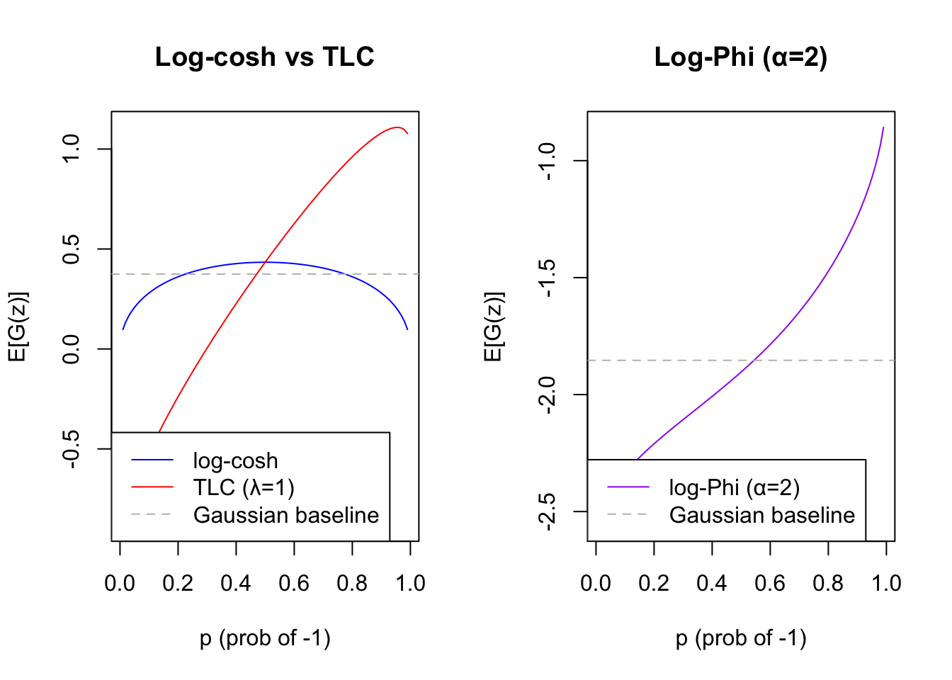
| Version | Author | Date |
|---|---|---|
| 7da05b8 | Matthew Stephens | 2026-07-16 |
par(mfrow = c(1, 1))Standard log-cosh falls below the Gaussian baseline for skewed sources. The tilted version increases monotonically toward the sparse extreme. Log-Phi exceeds the Gaussian baseline only for highly skewed sources (small \(p\), i.e., mostly positive projections), so it is suited to one-sided sparse sources.
Test 1: Symmetric binary source (k=1, p=0.5)
The simplest case: a single Rademacher source (-1 or +1 with equal probability). Both methods should work here since log-cosh peaks at p=0.5.
set.seed(10)
n = 200
p = 1000
k = 1
A = matrix(rnorm(p * k), nrow = p)
S_rad = matrix(sample(c(-1, 1), n, replace = TRUE), nrow = 1)
sigma = 0.1
X_rad = A %*% S_rad + matrix(rnorm(p * n, 0, sigma), nrow = p)
Z_rad = sqrt(n) * t(svd(X_rad)$v[, 1:k, drop = FALSE])

res_lc_rad     = run_seeds(Z_rad, S_rad, fastica_r1update,        compute_objective,        n_seeds = 50)
res_tlc_rad    = run_seeds(Z_rad, S_rad, fastica_r1update_tlc,    compute_objective_tlc,    n_seeds = 50)
res_logphi_rad = run_seeds(Z_rad, S_rad, fastica_r1update_logphi, compute_objective_logphi, n_seeds = 50)

cat("log-cosh  : mean max|cor| =", round(mean(res_lc_rad$maxcor),     3),
    " fraction > 0.9:", mean(res_lc_rad$maxcor     > 0.9), "\n")
log-cosh : mean max|cor| = 1 fraction > 0.9: 1 cat("tilted lc : mean max|cor| =", round(mean(res_tlc_rad$maxcor), 3),
" fraction > 0.9:", mean(res_tlc_rad$maxcor > 0.9), "\n")tilted lc : mean max|cor| = 1 fraction > 0.9: 1 cat("log-Phi : mean max|cor| =", round(mean(res_logphi_rad$maxcor), 3),
" fraction > 0.9:", mean(res_logphi_rad$maxcor > 0.9), "\n")log-Phi : mean max|cor| = 1 fraction > 0.9: 1 Test 2: Non-overlapping groups (k=4, p=0.25 per source)
Here we have 4 non-overlapping groups of 25 samples each in n=100, so each source is active for 25% of samples (p=0.25). Without noise the 4 groups would perfectly partition all samples, making the centered data rank k-1 and the k-th whitened component the constant direction. The added noise breaks this exact rank deficiency.
set.seed(1)
n = 100
p = 1000
k = 4
A = matrix(rnorm(p * k), nrow = p)
S = matrix(0, nrow = k, ncol = n)
S[1, 1:25]   = 1
S[2, 26:50]  = 1
S[3, 51:75]  = 1
S[4, 76:100] = 1
sigma = 0.1
X  = A %*% S + matrix(rnorm(p * n, 0, sigma), nrow = p)
Z  = prewhiten(X, k)

res_lc     = run_seeds(Z, S, fastica_r1update,        compute_objective)
res_tlc    = run_seeds(Z, S, fastica_r1update_tlc,    compute_objective_tlc)
res_logphi = run_seeds(Z, S, fastica_r1update_logphi, compute_objective_logphi)

par(mfrow = c(1, 3))
hist(res_lc$maxcor,     breaks = seq(0, 1, by = 0.05), main = "log-cosh",     xlab = "max |cor| with true S")
hist(res_tlc$maxcor,    breaks = seq(0, 1, by = 0.05), main = "tilted lc",    xlab = "max |cor| with true S")
hist(res_logphi$maxcor, breaks = seq(0, 1, by = 0.05), main = "log-Phi (α=2)", xlab = "max |cor| with true S")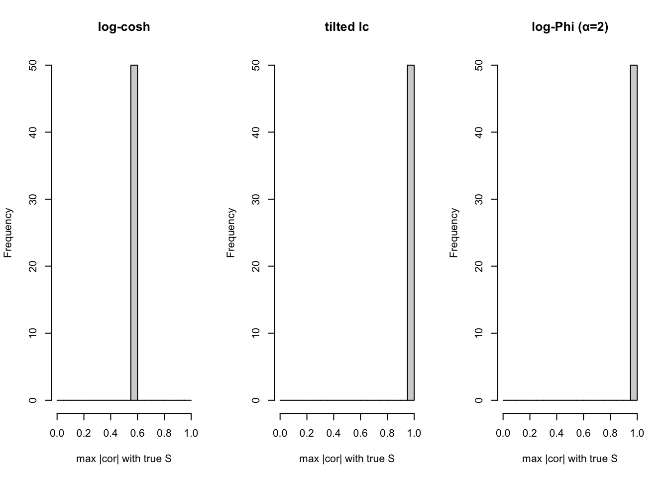
par(mfrow = c(1, 1))Best and worst seeds for tilted log-cosh on Test 2:
get_projection = function(X, seed, update_fn, n_iter = 200, ...) {
  set.seed(seed)
  w = rnorm(nrow(X))
  for (i in seq_len(n_iter))
    w = update_fn(X, w, ...)
  as.vector(t(X) %*% w)
}

best_seed  = which.max(res_tlc$maxcor)
worst_seed = which.min(res_tlc$maxcor)

proj_best  = get_projection(Z, best_seed,  fastica_r1update_tlc)
proj_worst = get_projection(Z, worst_seed, fastica_r1update_tlc)

par(mfrow = c(1, 2))
plot(proj_best,  main = paste0("TLC best seed (", best_seed, "), max|cor|=",
     round(res_tlc$maxcor[best_seed], 3)), xlab = "sample", ylab = "projection")
plot(proj_worst, main = paste0("TLC worst seed (", worst_seed, "), max|cor|=",
     round(res_tlc$maxcor[worst_seed], 3)), xlab = "sample", ylab = "projection")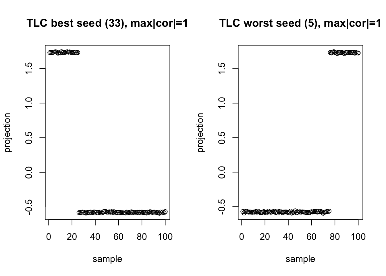
par(mfrow = c(1, 1))Test 3: Sparse binary sources (p=0.2)
Here the true source takes value 1 with probability 0.2. From the theoretical plot, p=0.2 is near where E[log(cosh(z))] is closest to the Gaussian baseline, making it hard for standard log-cosh to distinguish the source from Gaussian noise.
set.seed(2)
n   = 500
p   = 1000
k   = 4
prob_active = 0.2  # 20% of samples are "on" per source

A = matrix(rnorm(p * k), nrow = p)
S_sparse = matrix(0, nrow = k, ncol = n)
for (j in 1:k)
  S_sparse[j, sample(n, round(prob_active * n))] = 1

sigma = 0.1
X_sp = A %*% S_sparse + matrix(rnorm(p * n, 0, sigma), nrow = p)
Z_sp = prewhiten(X_sp, k)

res_lc_sp     = run_seeds(Z_sp, S_sparse, fastica_r1update,        compute_objective,        n_seeds = 100)
res_tlc_sp    = run_seeds(Z_sp, S_sparse, fastica_r1update_tlc,    compute_objective_tlc,    n_seeds = 100)
res_logphi_sp = run_seeds(Z_sp, S_sparse, fastica_r1update_logphi, compute_objective_logphi, n_seeds = 100)

cat("log-cosh:    mean max|cor| =", round(mean(res_lc_sp$maxcor),     3),
    " fraction > 0.9:", mean(res_lc_sp$maxcor     > 0.9), "\n")
log-cosh: mean max|cor| = 0.723 fraction > 0.9: 0.07 cat("tilted lc: mean max|cor| =", round(mean(res_tlc_sp$maxcor), 3),
" fraction > 0.9:", mean(res_tlc_sp$maxcor > 0.9), "\n")tilted lc: mean max|cor| = 1 fraction > 0.9: 1 cat("log-Phi: mean max|cor| =", round(mean(res_logphi_sp$maxcor), 3),
" fraction > 0.9:", mean(res_logphi_sp$maxcor > 0.9), "\n")log-Phi: mean max|cor| = 1 fraction > 0.9: 1 par(mfrow = c(1, 3))
hist(res_lc_sp$maxcor, breaks = seq(0, 1, by = 0.05),
main = "log-cosh", xlab = "max |cor| with true S")
hist(res_tlc_sp$maxcor, breaks = seq(0, 1, by = 0.05),
main = "tilted lc", xlab = "max |cor| with true S")
hist(res_logphi_sp$maxcor, breaks = seq(0, 1, by = 0.05),
main = "log-Phi (α=2)", xlab = "max |cor| with true S")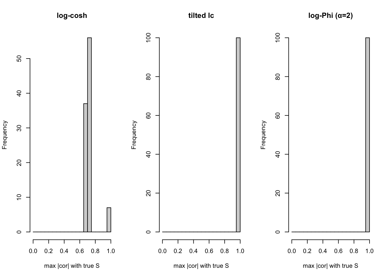
par(mfrow = c(1, 1))Multi-component extraction via deflation
To extract \(k\) components we use deflation: find one component at a time, then project it out of the weight space before searching for the next. Specifically, after finding weight vector \(w_1\), the next search is restricted to vectors orthogonal to \(w_1\) by subtracting the projection onto \(w_1\) after each update. This ensures each extracted component is distinct. We use multiple random starts per component and keep the one with the highest objective value.
fastica_deflation = function(X, k, update_fn, obj_fn, n_iter = 200, n_starts = 5, ...) {
  W = matrix(0, nrow(X), k)
  for (comp in seq_len(k)) {
    best_obj = -Inf
    best_w   = NULL
    for (s in seq_len(n_starts)) {
      set.seed(s + comp * 1000)
      w = rnorm(nrow(X))
      # project out already-found components
      if (comp > 1)
        w = w - W[, 1:(comp-1), drop=FALSE] %*% (t(W[, 1:(comp-1), drop=FALSE]) %*% w)
      w = w / sqrt(sum(w^2))
      for (i in seq_len(n_iter)) {
        w = update_fn(X, w, ...)
        # deflate
        if (comp > 1)
          w = w - W[, 1:(comp-1), drop=FALSE] %*% (t(W[, 1:(comp-1), drop=FALSE]) %*% w)
        w = w / sqrt(sum(w^2))
      }
      o = obj_fn(X, w, ...)
      if (o > best_obj) { best_obj = o; best_w = w }
    }
    W[, comp] = best_w
  }
  W
}

# Extract 4 components on the sparse simulation
W_lc     = fastica_deflation(Z_sp, k, fastica_r1update,        compute_objective)
W_tlc    = fastica_deflation(Z_sp, k, fastica_r1update_tlc,    compute_objective_tlc)
W_logphi = fastica_deflation(Z_sp, k, fastica_r1update_logphi, compute_objective_logphi)

cor_lc     = cor(t(S_sparse), t(Z_sp) %*% W_lc)
cor_tlc    = cor(t(S_sparse), t(Z_sp) %*% W_tlc)
cor_logphi = cor(t(S_sparse), t(Z_sp) %*% W_logphi)

cat("log-cosh deflation — max |cor| per true source:\n")
log-cosh deflation — max |cor| per true source:print(round(apply(abs(cor_lc), 1, max), 3))[1] 0.951 0.720 0.998 0.699cat("tilted log-cosh deflation — max |cor| per true source:\n")tilted log-cosh deflation — max |cor| per true source:print(round(apply(abs(cor_tlc), 1, max), 3))[1] 1.000 1.000 1.000 0.995cat("log-Phi deflation — max |cor| per true source:\n")log-Phi deflation — max |cor| per true source:print(round(apply(abs(cor_logphi), 1, max), 3))[1] 1.000 1.000 1.000 0.995Test 4: 9 overlapping groups, 20 members each, n=100
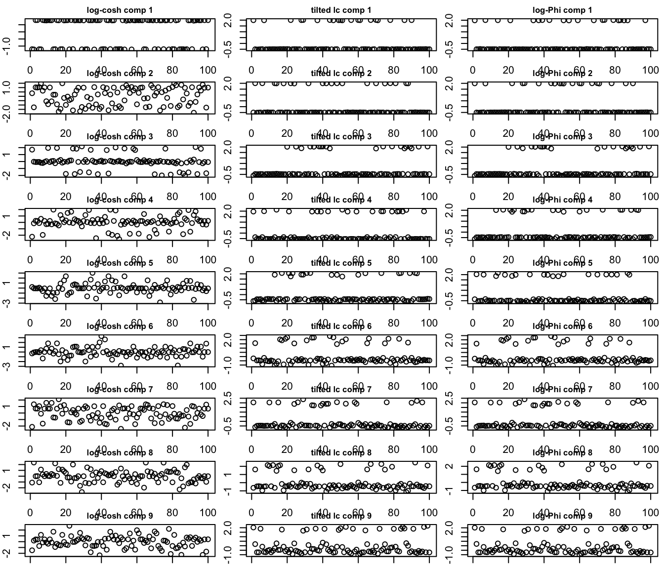
Here each source is active for 20 out of 100 samples (p=0.2), and groups can overlap. This is harder than the non-overlapping case and matches the simulation from the original file. We use deflation to extract all 9 components.
set.seed(1)
n = 100
p = 1000
K = 9
L = matrix(0, nrow = n, ncol = K)
for (i in 1:K) L[sample(n, 20), i] = 1
FF = matrix(rnorm(p * K), nrow = p, ncol = K)
sigma = 0.1
X9 = t(L %*% t(FF) + matrix(rnorm(n * p, 0, sigma), nrow = n))  # p x n
Z9 = prewhiten(X9, K)

W9_lc     = fastica_deflation(Z9, K, fastica_r1update,        compute_objective,        n_starts = 10)
W9_tlc    = fastica_deflation(Z9, K, fastica_r1update_tlc,    compute_objective_tlc,    n_starts = 10)
W9_logphi = fastica_deflation(Z9, K, fastica_r1update_logphi, compute_objective_logphi, n_starts = 10)

cor9_lc     = cor(L, t(Z9) %*% W9_lc)
cor9_tlc    = cor(L, t(Z9) %*% W9_tlc)
cor9_logphi = cor(L, t(Z9) %*% W9_logphi)

cat("log-cosh — max |cor| per true source:\n")
log-cosh — max |cor| per true source:print(round(apply(abs(cor9_lc), 2, max), 3))[1] 0.612 0.546 0.711 0.747 0.584 0.497 0.609 0.609 0.614cat("tilted log-cosh — max |cor| per true source:\n")tilted log-cosh — max |cor| per true source:print(round(apply(abs(cor9_tlc), 2, max), 3))[1] 1.000 1.000 0.998 0.998 0.996 0.975 0.990 0.968 0.954cat("log-Phi — max |cor| per true source:\n")log-Phi — max |cor| per true source:print(round(apply(abs(cor9_logphi), 2, max), 3))[1] 1.000 1.000 0.998 0.998 0.996 0.973 0.990 0.966 0.954Extracted sources (rows = components, columns = samples):
proj9_lc     = t(Z9) %*% W9_lc
proj9_tlc    = t(Z9) %*% W9_tlc
proj9_logphi = t(Z9) %*% W9_logphi

par(mfrow = c(K, 3), mar = c(1, 2, 1.5, 0.5))
for (i in 1:K) {
  plot(proj9_lc[, i],     main = paste0("log-cosh comp ", i),  ylab = "", xlab = "", cex.main = 0.8)
  plot(proj9_tlc[, i],    main = paste0("tilted lc comp ", i), ylab = "", xlab = "", cex.main = 0.8)
  plot(proj9_logphi[, i], main = paste0("log-Phi comp ", i),   ylab = "", xlab = "", cex.main = 0.8)
}
| Version | Author | Date |
|---|---|---|
| e64a684 | Matthew Stephens | 2026-07-16 |
par(mfrow = c(1, 1))Summary
The tilted log-cosh contrast G(z) = log(cosh(z)) + λz|z| addresses the fundamental failure of standard log-cosh for sparse binary sources. The odd term z|z| has expectation 2p−1, so sparse sources (p→1) score highly rather than falling below the Gaussian baseline.
The log-Phi contrast G(z) = log(Φ(αz)) is a one-sided function that rewards large positive projections. It exceeds the Gaussian baseline only when the source is highly skewed toward positive values (small p in the “prob of -1” convention), making it complementary to TLC for detecting asymmetric sparse sources.
sessionInfo()R version 4.4.2 (2024-10-31)
Platform: aarch64-apple-darwin20
Running under: macOS 26.5.2
Matrix products: default
BLAS: /System/Library/Frameworks/Accelerate.framework/Versions/A/Frameworks/vecLib.framework/Versions/A/libBLAS.dylib
LAPACK: /Library/Frameworks/R.framework/Versions/4.4-arm64/Resources/lib/libRlapack.dylib; LAPACK version 3.12.0
locale:
[1] en_US.UTF-8/en_US.UTF-8/en_US.UTF-8/C/en_US.UTF-8/en_US.UTF-8
time zone: America/Chicago
tzcode source: internal
attached base packages:
[1] stats graphics grDevices utils datasets methods base
loaded via a namespace (and not attached):
[1] vctrs_0.7.2 cli_3.6.5 knitr_1.51 rlang_1.1.7
[5] xfun_0.56 stringi_1.8.7 otel_0.2.0 promises_1.5.0
[9] jsonlite_2.0.0 workflowr_1.7.2 glue_1.8.0 rprojroot_2.1.1
[13] git2r_0.36.2 htmltools_0.5.9 httpuv_1.6.16 sass_0.4.10
[17] rmarkdown_2.30 jquerylib_0.1.4 evaluate_1.0.5 tibble_3.3.1
[21] fastmap_1.2.0 yaml_2.3.12 lifecycle_1.0.5 whisker_0.4.1
[25] stringr_1.6.0 compiler_4.4.2 fs_1.6.6 Rcpp_1.1.1
[29] pkgconfig_2.0.3 rstudioapi_0.18.0 later_1.4.6 digest_0.6.39
[33] R6_2.6.1 pillar_1.11.1 magrittr_2.0.4 bslib_0.10.0
[37] tools_4.4.2 cachem_1.1.0