mr.ash_ridge
Matthew Stephens
2020-05-19
Last updated: 2020-05-20
Checks: 7 0
Knit directory: misc/analysis/
This reproducible R Markdown analysis was created with workflowr (version 1.6.1). The Checks tab describes the reproducibility checks that were applied when the results were created. The Past versions tab lists the development history.
Great! Since the R Markdown file has been committed to the Git repository, you know the exact version of the code that produced these results.
Great job! The global environment was empty. Objects defined in the global environment can affect the analysis in your R Markdown file in unknown ways. For reproduciblity it’s best to always run the code in an empty environment.
The command set.seed(1) was run prior to running the code in the R Markdown file. Setting a seed ensures that any results that rely on randomness, e.g. subsampling or permutations, are reproducible.
Great job! Recording the operating system, R version, and package versions is critical for reproducibility.
Nice! There were no cached chunks for this analysis, so you can be confident that you successfully produced the results during this run.
Great job! Using relative paths to the files within your workflowr project makes it easier to run your code on other machines.
Great! You are using Git for version control. Tracking code development and connecting the code version to the results is critical for reproducibility.
The results in this page were generated with repository version 090e35d. See the Past versions tab to see a history of the changes made to the R Markdown and HTML files.
Note that you need to be careful to ensure that all relevant files for the analysis have been committed to Git prior to generating the results (you can use wflow_publish or wflow_git_commit). workflowr only checks the R Markdown file, but you know if there are other scripts or data files that it depends on. Below is the status of the Git repository when the results were generated:
Ignored files:
    Ignored:    .DS_Store
    Ignored:    .Rhistory
    Ignored:    .Rproj.user/
    Ignored:    analysis/.RData
    Ignored:    analysis/.Rhistory
    Ignored:    analysis/ALStruct_cache/
    Ignored:    data/.Rhistory
    Ignored:    data/pbmc/

Untracked files:
    Untracked:  .dropbox
    Untracked:  Icon
    Untracked:  analysis/GHstan.Rmd
    Untracked:  analysis/GTEX-cogaps.Rmd
    Untracked:  analysis/PACS.Rmd
    Untracked:  analysis/SPCAvRP.rmd
    Untracked:  analysis/admm_02.Rmd
    Untracked:  analysis/admm_03.Rmd
    Untracked:  analysis/compare-transformed-models.Rmd
    Untracked:  analysis/cormotif.Rmd
    Untracked:  analysis/cp_ash.Rmd
    Untracked:  analysis/eQTL.perm.rand.pdf
    Untracked:  analysis/eb_prepilot.Rmd
    Untracked:  analysis/eb_var.Rmd
    Untracked:  analysis/ebpmf1.Rmd
    Untracked:  analysis/flash_test_tree.Rmd
    Untracked:  analysis/ieQTL.perm.rand.pdf
    Untracked:  analysis/m6amash.Rmd
    Untracked:  analysis/mash_bhat_z.Rmd
    Untracked:  analysis/mash_ieqtl_permutations.Rmd
    Untracked:  analysis/mixsqp.Rmd
    Untracked:  analysis/mr_ash_modular.Rmd
    Untracked:  analysis/mr_ash_parameterization.Rmd
    Untracked:  analysis/mr_ash_pen.Rmd
    Untracked:  analysis/nejm.Rmd
    Untracked:  analysis/normalize.Rmd
    Untracked:  analysis/pbmc.Rmd
    Untracked:  analysis/poisson_transform.Rmd
    Untracked:  analysis/pseudodata.Rmd
    Untracked:  analysis/qrnotes.txt
    Untracked:  analysis/ridge_iterative_splitting.Rmd
    Untracked:  analysis/sc_bimodal.Rmd
    Untracked:  analysis/shrinkage_comparisons_changepoints.Rmd
    Untracked:  analysis/susie_en.Rmd
    Untracked:  analysis/susie_z_investigate.Rmd
    Untracked:  analysis/svd-timing.Rmd
    Untracked:  analysis/temp.Rmd
    Untracked:  analysis/test-figure/
    Untracked:  analysis/test.Rmd
    Untracked:  analysis/test.Rpres
    Untracked:  analysis/test.md
    Untracked:  analysis/test_qr.R
    Untracked:  analysis/test_sparse.Rmd
    Untracked:  analysis/z.txt
    Untracked:  code/multivariate_testfuncs.R
    Untracked:  code/rqb.hacked.R
    Untracked:  data/4matthew/
    Untracked:  data/4matthew2/
    Untracked:  data/E-MTAB-2805.processed.1/
    Untracked:  data/ENSG00000156738.Sim_Y2.RDS
    Untracked:  data/GDS5363_full.soft.gz
    Untracked:  data/GSE41265_allGenesTPM.txt
    Untracked:  data/Muscle_Skeletal.ACTN3.pm1Mb.RDS
    Untracked:  data/Thyroid.FMO2.pm1Mb.RDS
    Untracked:  data/bmass.HaemgenRBC2016.MAF01.Vs2.MergedDataSources.200kRanSubset.ChrBPMAFMarkerZScores.vs1.txt.gz
    Untracked:  data/bmass.HaemgenRBC2016.Vs2.NewSNPs.ZScores.hclust.vs1.txt
    Untracked:  data/bmass.HaemgenRBC2016.Vs2.PreviousSNPs.ZScores.hclust.vs1.txt
    Untracked:  data/eb_prepilot/
    Untracked:  data/finemap_data/fmo2.sim/b.txt
    Untracked:  data/finemap_data/fmo2.sim/dap_out.txt
    Untracked:  data/finemap_data/fmo2.sim/dap_out2.txt
    Untracked:  data/finemap_data/fmo2.sim/dap_out2_snp.txt
    Untracked:  data/finemap_data/fmo2.sim/dap_out_snp.txt
    Untracked:  data/finemap_data/fmo2.sim/data
    Untracked:  data/finemap_data/fmo2.sim/fmo2.sim.config
    Untracked:  data/finemap_data/fmo2.sim/fmo2.sim.k
    Untracked:  data/finemap_data/fmo2.sim/fmo2.sim.k4.config
    Untracked:  data/finemap_data/fmo2.sim/fmo2.sim.k4.snp
    Untracked:  data/finemap_data/fmo2.sim/fmo2.sim.ld
    Untracked:  data/finemap_data/fmo2.sim/fmo2.sim.snp
    Untracked:  data/finemap_data/fmo2.sim/fmo2.sim.z
    Untracked:  data/finemap_data/fmo2.sim/pos.txt
    Untracked:  data/logm.csv
    Untracked:  data/m.cd.RDS
    Untracked:  data/m.cdu.old.RDS
    Untracked:  data/m.new.cd.RDS
    Untracked:  data/m.old.cd.RDS
    Untracked:  data/mainbib.bib.old
    Untracked:  data/mat.csv
    Untracked:  data/mat.txt
    Untracked:  data/mat_new.csv
    Untracked:  data/matrix_lik.rds
    Untracked:  data/paintor_data/
    Untracked:  data/temp.txt
    Untracked:  data/y.txt
    Untracked:  data/y_f.txt
    Untracked:  data/zscore_jointLCLs_m6AQTLs_susie_eQTLpruned.rds
    Untracked:  data/zscore_jointLCLs_random.rds
    Untracked:  explore_udi.R
    Untracked:  output/fit.k10.rds
    Untracked:  output/fit.varbvs.RDS
    Untracked:  output/glmnet.fit.RDS
    Untracked:  output/test.bv.txt
    Untracked:  output/test.gamma.txt
    Untracked:  output/test.hyp.txt
    Untracked:  output/test.log.txt
    Untracked:  output/test.param.txt
    Untracked:  output/test2.bv.txt
    Untracked:  output/test2.gamma.txt
    Untracked:  output/test2.hyp.txt
    Untracked:  output/test2.log.txt
    Untracked:  output/test2.param.txt
    Untracked:  output/test3.bv.txt
    Untracked:  output/test3.gamma.txt
    Untracked:  output/test3.hyp.txt
    Untracked:  output/test3.log.txt
    Untracked:  output/test3.param.txt
    Untracked:  output/test4.bv.txt
    Untracked:  output/test4.gamma.txt
    Untracked:  output/test4.hyp.txt
    Untracked:  output/test4.log.txt
    Untracked:  output/test4.param.txt
    Untracked:  output/test5.bv.txt
    Untracked:  output/test5.gamma.txt
    Untracked:  output/test5.hyp.txt
    Untracked:  output/test5.log.txt
    Untracked:  output/test5.param.txt

Unstaged changes:
    Modified:   analysis/ash_delta_operator.Rmd
    Modified:   analysis/ash_pois_bcell.Rmd
    Modified:   analysis/minque.Rmd
    Modified:   analysis/mr_missing_data.Rmd
Note that any generated files, e.g. HTML, png, CSS, etc., are not included in this status report because it is ok for generated content to have uncommitted changes.
These are the previous versions of the repository in which changes were made to the R Markdown (analysis/mr.ash_ridge.Rmd) and HTML (docs/mr.ash_ridge.html) files. If you’ve configured a remote Git repository (see ?wflow_git_remote), click on the hyperlinks in the table below to view the files as they were in that past version.
| File | Version | Author | Date | Message |
|---|---|---|---|---|
| Rmd | 090e35d | Matthew Stephens | 2020-05-20 | wflow_publish(“mr.ash_ridge.Rmd”) |
library("mr.ash.alpha")Introduction
My idea here is to experiment with a new model \[y=Xb + e\] where \(b_j = (b_1)_j (b_2)_j\). My initial idea was to have elements of \(b_1\) having ridge (normal) prior and elements of \(b_2\) having ash prior. However, it turns out to be interesting, perhaps even more interesting, to use ridge priors for both, and to further extend to \(b_j \prod_k (b_k)_j\).
In any case the motivation is that we can do variational approximation \(q(b_1)\prod q_j(b_2j)\) where \(q(b_1)\) does not factorize - it is a full approximation on all \(p\) (which is tractible due to the normal prior). So it can capture dependence among \(b\) values.
In the non-sparse case we would expect the EB estimation of ash prior to end up fitting a normal, so in that case \(b_j\) will be a product of two normals. So this model does not include ridge regression as a special case.
However, a product of two normals actually has quite an interesting shape:
hist(rnorm(10000)*rnorm(10000),nclass=100)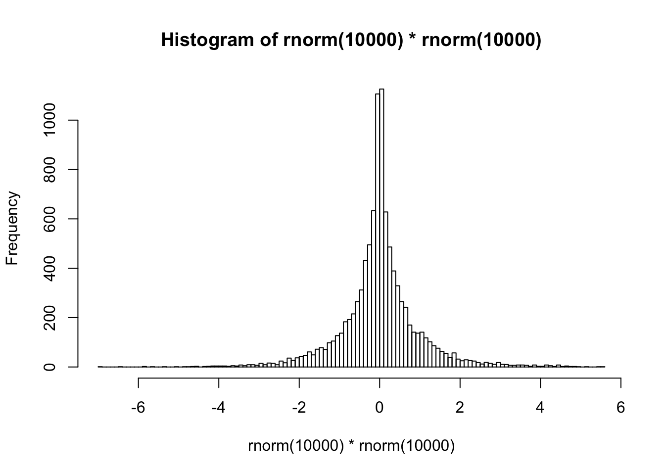 This is perhaps not a bad “null” non-sparse model in itself.
Fitting
I think we can do the regular variational thing for this model, but for now to get something working quickly I’m going to do a simple 2-stage procedure: fit ridge regression on it’s own to estimate \(b_1\), and then fit ash to \(y=(XB_1) b_2+e\) where \(B_1\) is the diagonal matrix with estimated \(b_1\) on it’s diagonal.
We will try a challenging trend-filtering example (challenging partly as it has highly correlated covariates):
set.seed(100)
sd = 1
n = 100
p = n
X = matrix(0,nrow=n,ncol=n)
for(i in 1:n){
  X[i:n,i] = 1:(n-i+1)
}
btrue = rep(0,n)
btrue[40] = 8
btrue[41] = -8
Y = X %*% btrue + sd*rnorm(n)

plot(Y)
lines(X %*% btrue)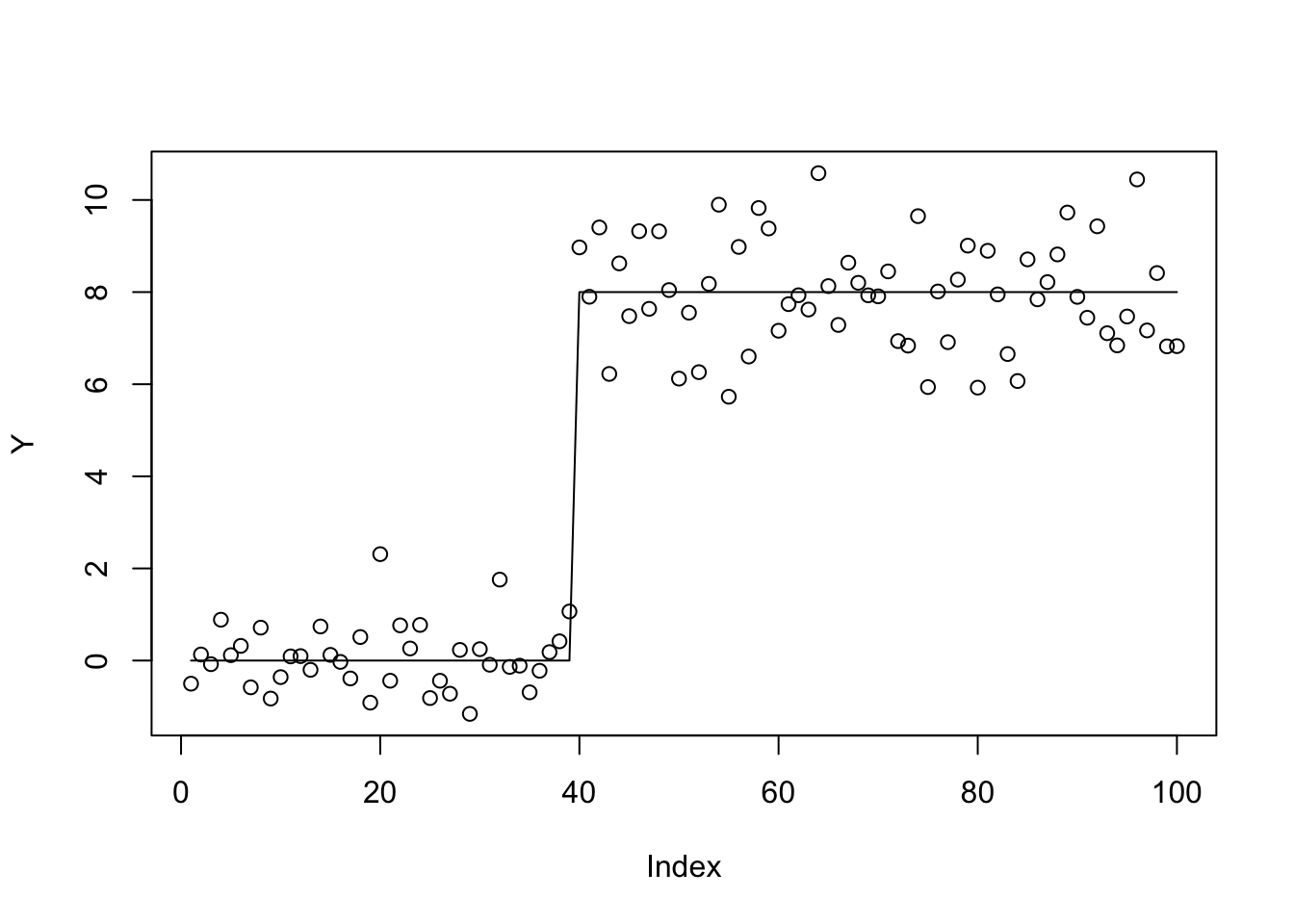
First a function to compute the ridge posterior If \(b_j \sim N(0,s_b^2)\) then \(Y \sim N(0, s^2 I_n + s_b^2(XX'))\).
ridge = function(y,A,prior_variance,prior_mean=rep(0,ncol(A)),residual_variance=1){
  n = length(y)
  p = ncol(A)
  L = chol(t(A) %*% A + (residual_variance/prior_variance)*diag(p))
  b = backsolve(L, t(A) %*% y + (residual_variance/prior_variance)*prior_mean, transpose=TRUE)
  b = backsolve(L, b)
  #b = chol2inv(L) %*% (t(A) %*% y + (residual_variance/prior_variance)*prior_mean)
  return(b)
}
Plot the ridge fit- looks OK ish.
plot(Y)
b_ridge = ridge(Y,X,10)
lines(X %*% b_ridge)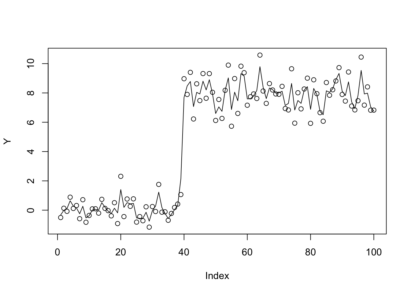
Apply mr.ash regularly - it does poorly, perhaps (in part) because initialization with glmnet is not very good here.
fit.mrash = mr.ash(X,Y,standardize=FALSE)
plot(Y)
lines(X %*% fit.mrash$beta,col=2)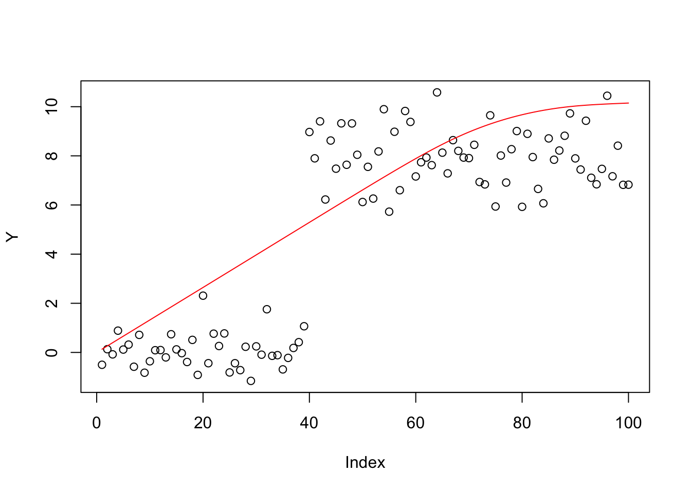
Try initializing to the ridge fit:
fit.mrash = mr.ash(X,Y,standardize=FALSE,beta.init = b_ridge)
plot(Y)
lines(X %*% fit.mrash$beta,col=3)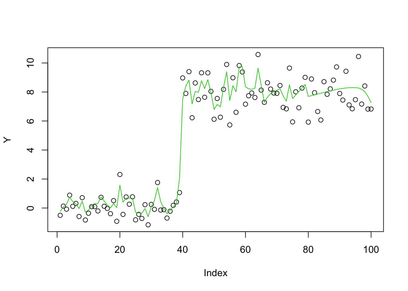
Now apply mr.ash with \(X\) scaled by the ridge fit, as suggested above, initializing at 1.
X_scale = t(t(X) * as.vector(b_ridge))
fit.mrash = mr.ash(X_scale,Y,standardize=FALSE,beta.init = rep(1,100),sigma2=1,update.sigma=FALSE)
plot(Y)
lines(X %*% (as.vector(b_ridge)*fit.mrash$beta),col=4)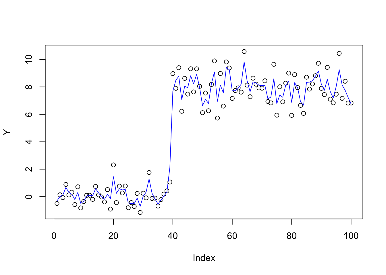
It didn’t really change much, which is a bit disappointing. Try iterating:
X_scale = t(t(X) * as.vector(fit.mrash$beta))
b_ridge = ridge(Y,X_scale,1,1)
X_scale = t(t(X) * as.vector(b_ridge))
fit.mrash = mr.ash(X_scale,Y,standardize=FALSE,beta.init = rep(1,100))

plot(Y)
lines(X %*% (as.vector(b_ridge)*fit.mrash$beta),col=4)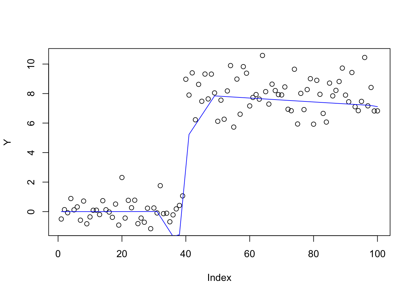
Iterative ridge regression
So that initial try didn’t work as well as I hoped. There is probably more investigation to be done, but I tried something different, based on \(b_j \prod_k (b_k)_j\) where each \(b_k\) has a ridge prior, so \(b_j\) is a product of gaussians.
Note that product of gaussians becomes sparser and longer tailed the more you use:
hist(rnorm(1000)*rnorm(1000)*rnorm(1000)*rnorm(1000),nclass=100)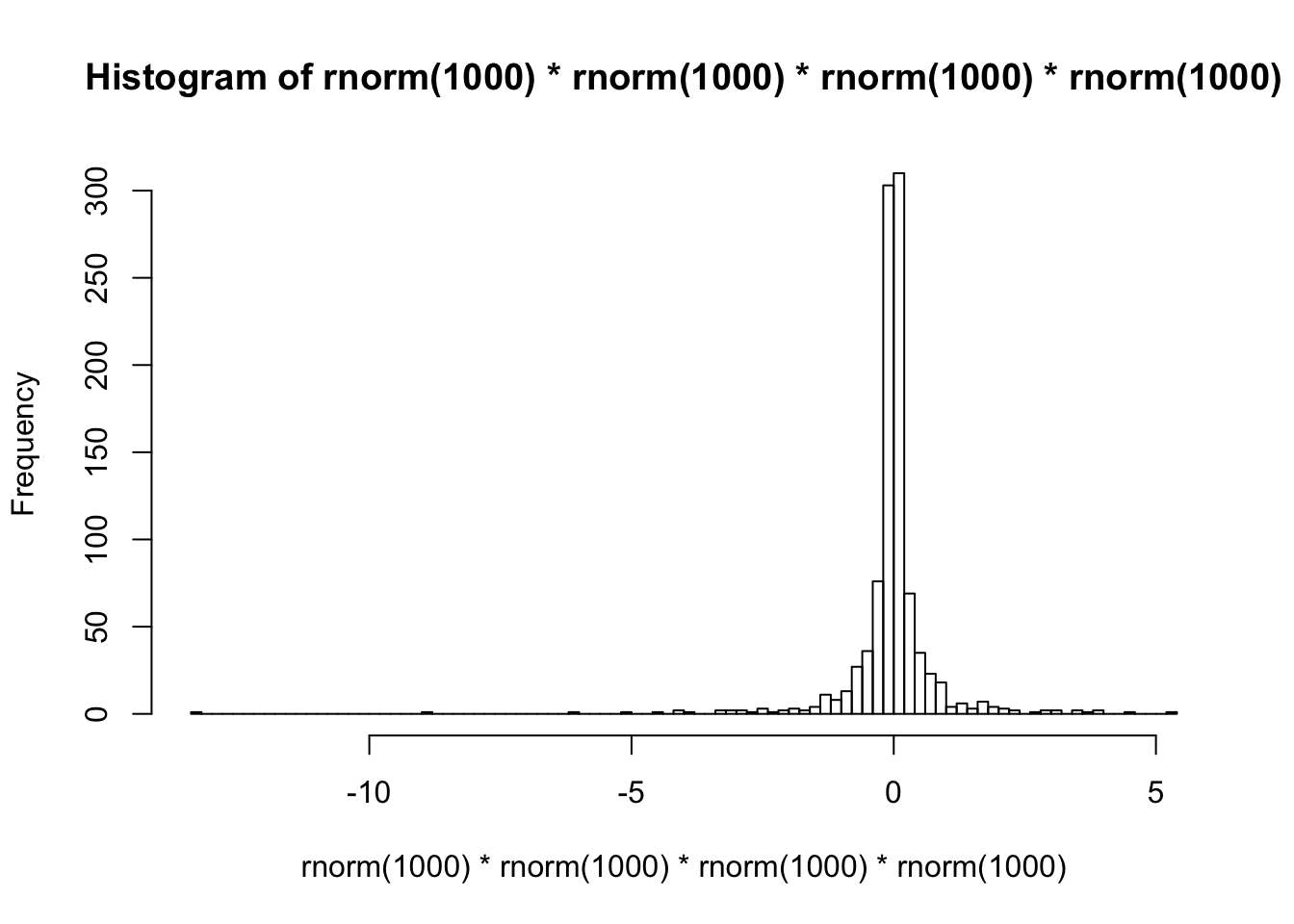
So iteration is a way of using ridge regression to induce sparsity…
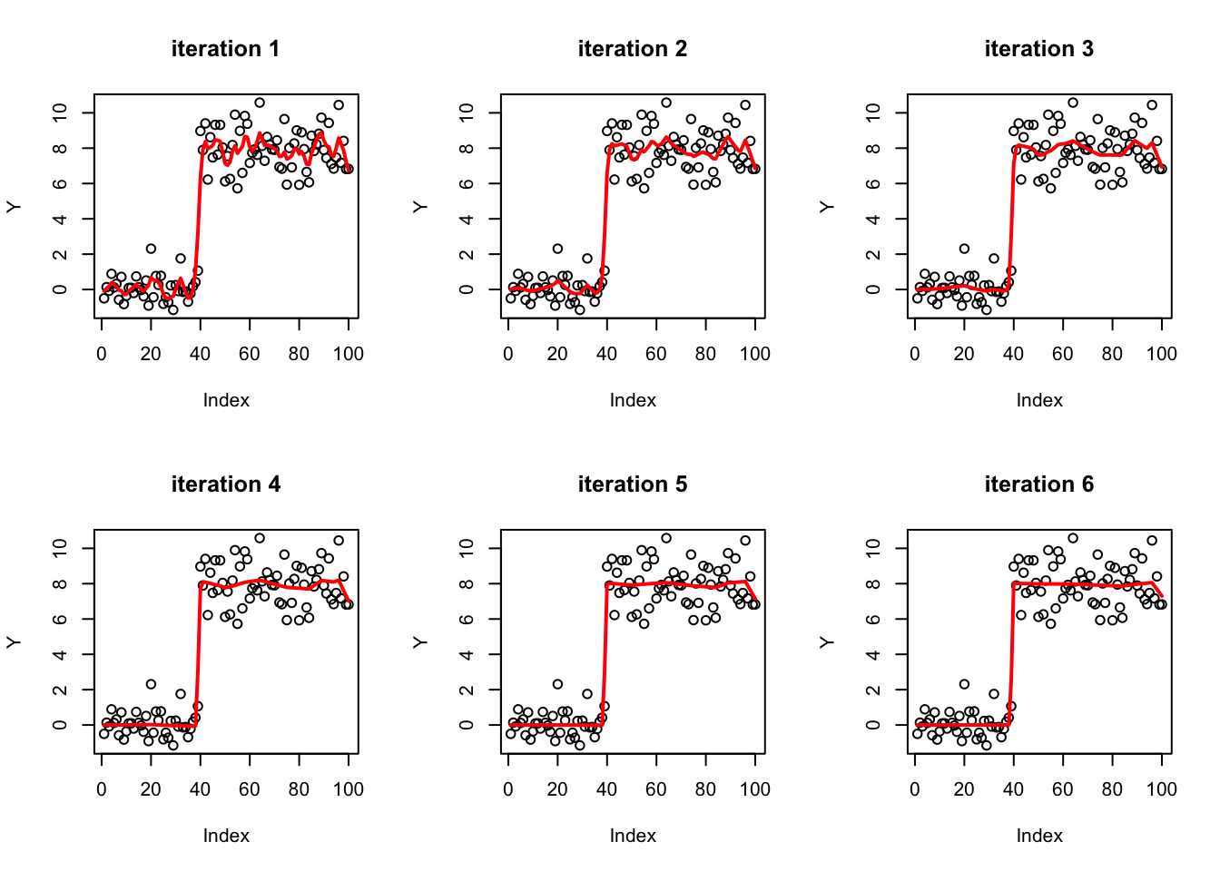
Here I try iterating 3 times, and you can see the fit becomes gradually “sparser” (sparse solutions are piecewise linear in this basis). (Note: throughout I fix the ridge prior variance to 1, which is not necessarily optimal…)
b_curr = ridge(Y,X,1)
par(mfrow=c(2,3))
plot(Y,main=paste0("iteration ",1))
lines(X %*% b_curr,col=2,lwd=2)

for(i in 2:6){
  X_scale = t(t(X) * as.vector(b_curr))
  b_ridge = ridge(Y,X_scale,1)
  b_curr = b_curr*b_ridge
  plot(Y,main=paste0("iteration ",i))
  lines(X %*% b_curr,col=2,lwd=2)
}
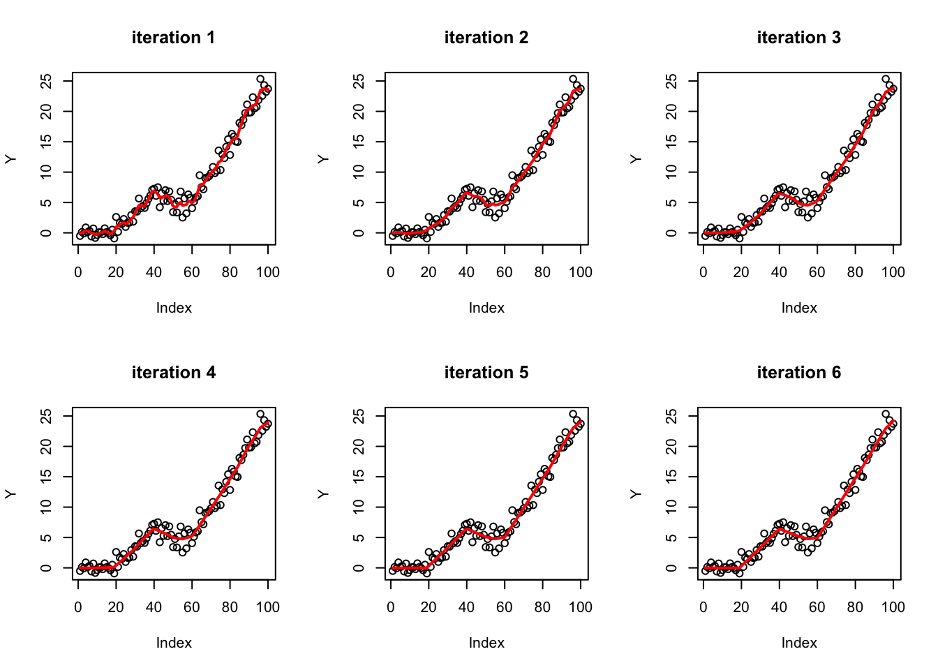
Try another example
set.seed(100)
sd = 1
n = 100
p = n
X = matrix(0,nrow=n,ncol=n)
for(i in 1:n){
  X[i:n,i] = 1:(n-i+1)
}
btrue = rep(0,n)
btrue[20] = .3
btrue[41] = -.4
btrue[60]= .6
Y = X %*% btrue + sd*rnorm(n)
b_curr = ridge(Y,X,1)
par(mfrow=c(2,3))
plot(Y,main=paste0("iteration ",1))
lines(X %*% b_curr,col=2,lwd=2)
for(i in 2:6){
X_scale = t(t(X) * as.vector(b_curr))
b_ridge = ridge(Y,X_scale,1)
b_curr = b_curr*b_ridge
plot(Y,main=paste0("iteration ",i))
lines(X %*% b_curr,col=2,lwd=2)
}
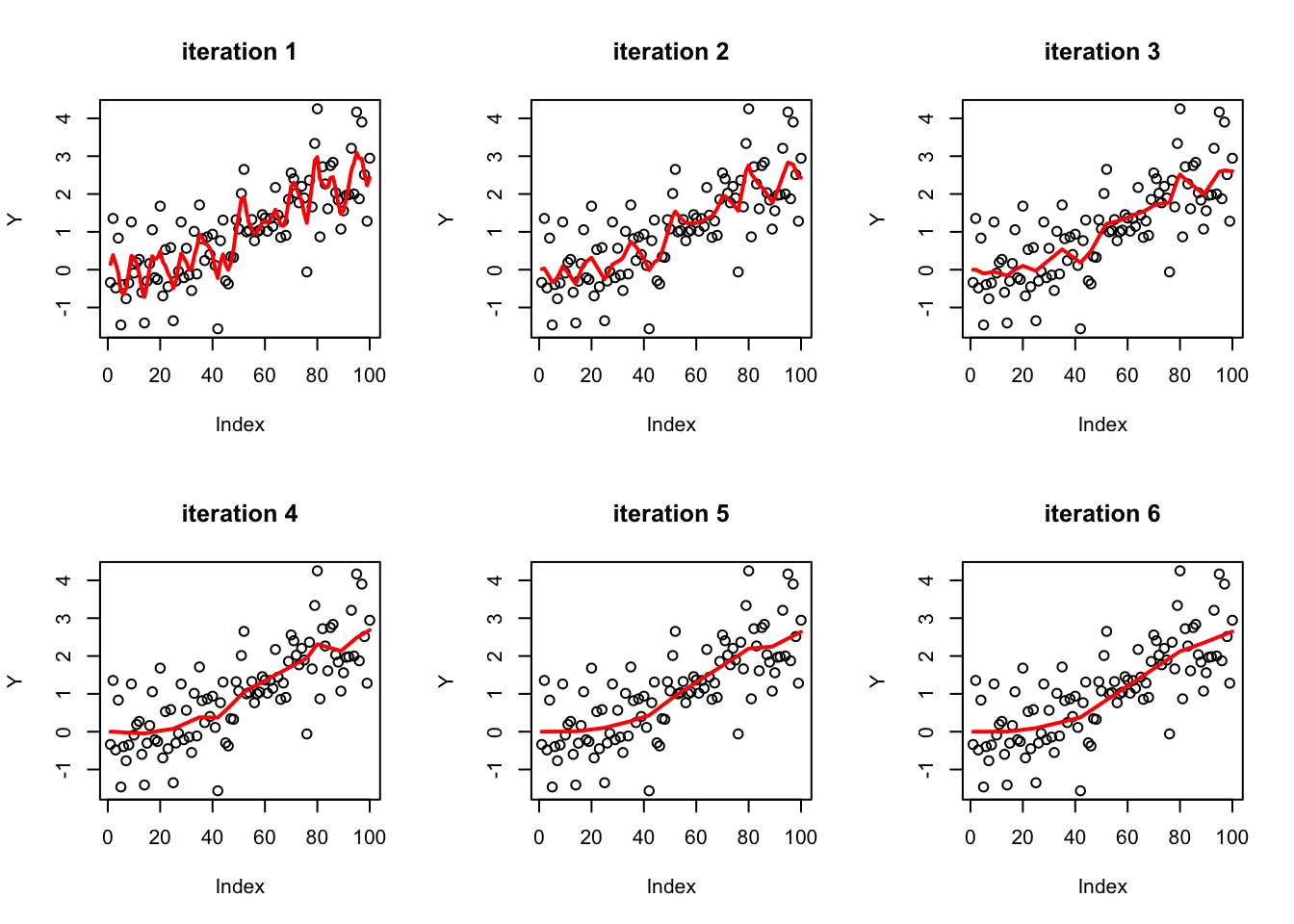
A non-sparse example
The above examples are both sparse. We try a non-sparse example here.
set.seed(100)
sd = 1
n = 100
p = n
X = matrix(0,nrow=n,ncol=n)
for(i in 1:n){
  X[i:n,i] = 1:(n-i+1)
}
btrue = rep(0,n)
btrue = rnorm(n,0,0.01)
Y = X %*% btrue + sd*rnorm(n)
b_curr = ridge(Y,X,1)
par(mfrow=c(2,3))
plot(Y,main=paste0("iteration ",1))
lines(X %*% b_curr,col=2,lwd=2)
for(i in 2:6){
X_scale = t(t(X) * as.vector(b_curr))
b_ridge = ridge(Y,X_scale,1)
b_curr = b_curr*b_ridge
plot(Y,main=paste0("iteration ",i))
lines(X %*% b_curr,col=2,lwd=2)
}
Summary
I found these results pretty interesting and promising, although very preliminary. Things to do: work out the proper variational approximation, and learn ridge mean and variance by EB. (Note if we allow mean=1 in ridge prior, the it can learn mean=1, variance=0 and the fitting process can stop…)
sessionInfo()R version 3.6.0 (2019-04-26)
Platform: x86_64-apple-darwin15.6.0 (64-bit)
Running under: macOS Mojave 10.14.6
Matrix products: default
BLAS: /Library/Frameworks/R.framework/Versions/3.6/Resources/lib/libRblas.0.dylib
LAPACK: /Library/Frameworks/R.framework/Versions/3.6/Resources/lib/libRlapack.dylib
locale:
[1] en_US.UTF-8/en_US.UTF-8/en_US.UTF-8/C/en_US.UTF-8/en_US.UTF-8
attached base packages:
[1] stats graphics grDevices utils datasets methods base
other attached packages:
[1] mr.ash.alpha_0.1-7
loaded via a namespace (and not attached):
[1] workflowr_1.6.1 Rcpp_1.0.4.6 lattice_0.20-40 rprojroot_1.3-2
[5] digest_0.6.25 later_1.0.0 grid_3.6.0 R6_2.4.1
[9] backports_1.1.5 git2r_0.26.1 magrittr_1.5 evaluate_0.14
[13] stringi_1.4.6 rlang_0.4.5 fs_1.3.2 promises_1.1.0
[17] whisker_0.4 Matrix_1.2-18 rmarkdown_2.1 tools_3.6.0
[21] stringr_1.4.0 glue_1.4.0 httpuv_1.5.2 xfun_0.12
[25] yaml_2.2.1 compiler_3.6.0 htmltools_0.4.0 knitr_1.28