mr_ash_vs_lasso
Matthew Stephens
2020-06-12
Last updated: 2021-01-15
Checks: 7 0
Knit directory: misc/analysis/
This reproducible R Markdown analysis was created with workflowr (version 1.6.2). The Checks tab describes the reproducibility checks that were applied when the results were created. The Past versions tab lists the development history.
Great! Since the R Markdown file has been committed to the Git repository, you know the exact version of the code that produced these results.
Great job! The global environment was empty. Objects defined in the global environment can affect the analysis in your R Markdown file in unknown ways. For reproduciblity it’s best to always run the code in an empty environment.
The command set.seed(1) was run prior to running the code in the R Markdown file. Setting a seed ensures that any results that rely on randomness, e.g. subsampling or permutations, are reproducible.
Great job! Recording the operating system, R version, and package versions is critical for reproducibility.
Nice! There were no cached chunks for this analysis, so you can be confident that you successfully produced the results during this run.
Great job! Using relative paths to the files within your workflowr project makes it easier to run your code on other machines.
Great! You are using Git for version control. Tracking code development and connecting the code version to the results is critical for reproducibility.
The results in this page were generated with repository version 1134186. See the Past versions tab to see a history of the changes made to the R Markdown and HTML files.
Note that you need to be careful to ensure that all relevant files for the analysis have been committed to Git prior to generating the results (you can use wflow_publish or wflow_git_commit). workflowr only checks the R Markdown file, but you know if there are other scripts or data files that it depends on. Below is the status of the Git repository when the results were generated:
Ignored files:
    Ignored:    .DS_Store
    Ignored:    .Rhistory
    Ignored:    .Rproj.user/
    Ignored:    analysis/.RData
    Ignored:    analysis/.Rhistory
    Ignored:    analysis/ALStruct_cache/
    Ignored:    data/.Rhistory
    Ignored:    data/pbmc/

Untracked files:
    Untracked:  .dropbox
    Untracked:  Icon
    Untracked:  analysis/GHstan.Rmd
    Untracked:  analysis/GTEX-cogaps.Rmd
    Untracked:  analysis/PACS.Rmd
    Untracked:  analysis/Rplot.png
    Untracked:  analysis/SPCAvRP.rmd
    Untracked:  analysis/admm_02.Rmd
    Untracked:  analysis/admm_03.Rmd
    Untracked:  analysis/compare-transformed-models.Rmd
    Untracked:  analysis/cormotif.Rmd
    Untracked:  analysis/cp_ash.Rmd
    Untracked:  analysis/eQTL.perm.rand.pdf
    Untracked:  analysis/eb_prepilot.Rmd
    Untracked:  analysis/eb_var.Rmd
    Untracked:  analysis/ebpmf1.Rmd
    Untracked:  analysis/flash_test_tree.Rmd
    Untracked:  analysis/flash_tree.Rmd
    Untracked:  analysis/ieQTL.perm.rand.pdf
    Untracked:  analysis/lasso_em_03.Rmd
    Untracked:  analysis/m6amash.Rmd
    Untracked:  analysis/mash_bhat_z.Rmd
    Untracked:  analysis/mash_ieqtl_permutations.Rmd
    Untracked:  analysis/mixsqp.Rmd
    Untracked:  analysis/mr.ash_lasso_init.Rmd
    Untracked:  analysis/mr.mash.test.Rmd
    Untracked:  analysis/mr_ash_modular.Rmd
    Untracked:  analysis/mr_ash_parameterization.Rmd
    Untracked:  analysis/mr_ash_pen.Rmd
    Untracked:  analysis/mr_ash_ridge.Rmd
    Untracked:  analysis/nejm.Rmd
    Untracked:  analysis/nmf_bg.Rmd
    Untracked:  analysis/normal_conditional_on_r2.Rmd
    Untracked:  analysis/normalize.Rmd
    Untracked:  analysis/pbmc.Rmd
    Untracked:  analysis/poisson_transform.Rmd
    Untracked:  analysis/pseudodata.Rmd
    Untracked:  analysis/qrnotes.txt
    Untracked:  analysis/ridge_iterative_02.Rmd
    Untracked:  analysis/ridge_iterative_splitting.Rmd
    Untracked:  analysis/samps/
    Untracked:  analysis/sc_bimodal.Rmd
    Untracked:  analysis/shrinkage_comparisons_changepoints.Rmd
    Untracked:  analysis/susie_en.Rmd
    Untracked:  analysis/susie_z_investigate.Rmd
    Untracked:  analysis/svd-timing.Rmd
    Untracked:  analysis/temp.RDS
    Untracked:  analysis/temp.Rmd
    Untracked:  analysis/test-figure/
    Untracked:  analysis/test.Rmd
    Untracked:  analysis/test.Rpres
    Untracked:  analysis/test.md
    Untracked:  analysis/test_qr.R
    Untracked:  analysis/test_sparse.Rmd
    Untracked:  analysis/z.txt
    Untracked:  code/multivariate_testfuncs.R
    Untracked:  code/rqb.hacked.R
    Untracked:  data/4matthew/
    Untracked:  data/4matthew2/
    Untracked:  data/E-MTAB-2805.processed.1/
    Untracked:  data/ENSG00000156738.Sim_Y2.RDS
    Untracked:  data/GDS5363_full.soft.gz
    Untracked:  data/GSE41265_allGenesTPM.txt
    Untracked:  data/Muscle_Skeletal.ACTN3.pm1Mb.RDS
    Untracked:  data/Thyroid.FMO2.pm1Mb.RDS
    Untracked:  data/bmass.HaemgenRBC2016.MAF01.Vs2.MergedDataSources.200kRanSubset.ChrBPMAFMarkerZScores.vs1.txt.gz
    Untracked:  data/bmass.HaemgenRBC2016.Vs2.NewSNPs.ZScores.hclust.vs1.txt
    Untracked:  data/bmass.HaemgenRBC2016.Vs2.PreviousSNPs.ZScores.hclust.vs1.txt
    Untracked:  data/eb_prepilot/
    Untracked:  data/finemap_data/fmo2.sim/b.txt
    Untracked:  data/finemap_data/fmo2.sim/dap_out.txt
    Untracked:  data/finemap_data/fmo2.sim/dap_out2.txt
    Untracked:  data/finemap_data/fmo2.sim/dap_out2_snp.txt
    Untracked:  data/finemap_data/fmo2.sim/dap_out_snp.txt
    Untracked:  data/finemap_data/fmo2.sim/data
    Untracked:  data/finemap_data/fmo2.sim/fmo2.sim.config
    Untracked:  data/finemap_data/fmo2.sim/fmo2.sim.k
    Untracked:  data/finemap_data/fmo2.sim/fmo2.sim.k4.config
    Untracked:  data/finemap_data/fmo2.sim/fmo2.sim.k4.snp
    Untracked:  data/finemap_data/fmo2.sim/fmo2.sim.ld
    Untracked:  data/finemap_data/fmo2.sim/fmo2.sim.snp
    Untracked:  data/finemap_data/fmo2.sim/fmo2.sim.z
    Untracked:  data/finemap_data/fmo2.sim/pos.txt
    Untracked:  data/logm.csv
    Untracked:  data/m.cd.RDS
    Untracked:  data/m.cdu.old.RDS
    Untracked:  data/m.new.cd.RDS
    Untracked:  data/m.old.cd.RDS
    Untracked:  data/mainbib.bib.old
    Untracked:  data/mat.csv
    Untracked:  data/mat.txt
    Untracked:  data/mat_new.csv
    Untracked:  data/matrix_lik.rds
    Untracked:  data/paintor_data/
    Untracked:  data/running_data_chris.csv
    Untracked:  data/running_data_matthew.csv
    Untracked:  data/temp.txt
    Untracked:  data/y.txt
    Untracked:  data/y_f.txt
    Untracked:  data/zscore_jointLCLs_m6AQTLs_susie_eQTLpruned.rds
    Untracked:  data/zscore_jointLCLs_random.rds
    Untracked:  explore_udi.R
    Untracked:  output/fit.k10.rds
    Untracked:  output/fit.varbvs.RDS
    Untracked:  output/glmnet.fit.RDS
    Untracked:  output/test.bv.txt
    Untracked:  output/test.gamma.txt
    Untracked:  output/test.hyp.txt
    Untracked:  output/test.log.txt
    Untracked:  output/test.param.txt
    Untracked:  output/test2.bv.txt
    Untracked:  output/test2.gamma.txt
    Untracked:  output/test2.hyp.txt
    Untracked:  output/test2.log.txt
    Untracked:  output/test2.param.txt
    Untracked:  output/test3.bv.txt
    Untracked:  output/test3.gamma.txt
    Untracked:  output/test3.hyp.txt
    Untracked:  output/test3.log.txt
    Untracked:  output/test3.param.txt
    Untracked:  output/test4.bv.txt
    Untracked:  output/test4.gamma.txt
    Untracked:  output/test4.hyp.txt
    Untracked:  output/test4.log.txt
    Untracked:  output/test4.param.txt
    Untracked:  output/test5.bv.txt
    Untracked:  output/test5.gamma.txt
    Untracked:  output/test5.hyp.txt
    Untracked:  output/test5.log.txt
    Untracked:  output/test5.param.txt

Unstaged changes:
    Modified:   analysis/ash_delta_operator.Rmd
    Modified:   analysis/ash_pois_bcell.Rmd
    Modified:   analysis/lasso_em.Rmd
    Modified:   analysis/minque.Rmd
    Modified:   analysis/mr_missing_data.Rmd
    Modified:   analysis/ridge_admm.Rmd
Note that any generated files, e.g. HTML, png, CSS, etc., are not included in this status report because it is ok for generated content to have uncommitted changes.
These are the previous versions of the repository in which changes were made to the R Markdown (analysis/mr_ash_vs_lasso.Rmd) and HTML (docs/mr_ash_vs_lasso.html) files. If you’ve configured a remote Git repository (see ?wflow_git_remote), click on the hyperlinks in the table below to view the files as they were in that past version.
| File | Version | Author | Date | Message |
|---|---|---|---|---|
| Rmd | 1134186 | Matthew Stephens | 2021-01-15 | workflowr::wflow_publish(“analysis/mr_ash_vs_lasso.Rmd”) |
| html | d7157a8 | Matthew Stephens | 2020-06-19 | Build site. |
| Rmd | f8037eb | Matthew Stephens | 2020-06-19 | workflowr::wflow_publish(“mr_ash_vs_lasso.Rmd”) |
| html | c94d7bf | Matthew Stephens | 2020-06-12 | Build site. |
| Rmd | 94bd508 | Matthew Stephens | 2020-06-12 | workflowr::wflow_publish(“mr_ash_vs_lasso.Rmd”) |
library("mr.ash.alpha")
library("glmnet")
Warning: package 'glmnet' was built under R version 3.6.2Loading required package: MatrixLoaded glmnet 4.1Introduction
This is to illustrate a setting where Fabio Morgante found lasso to work better than mr.ash. The simulation is based on his set-up, and then simplified. (Note that I have set the columns of \(X\) to have norm approximately 1 to make connections with the mr.ash paper easier.)
I ran mr.ash with both estimating the prior and fixing the prior (and residual variance) to the true value. I initialized from the solution obtained by lasso from glmnet. I compare the mean squared errors. With estimated prior mr ash is consistently worse than lasso. With the correct prior the performance is closer, but still usually worse.
  set.seed(123)
  n <- 500
  p <- 1000
  p_causal <- 500 # number of causal variables (simulated effects N(0,1))
  pve <- 0.95
  nrep = 10
  rmse_mrash = rep(0,nrep)
  rmse_glmnet = rep(0,nrep)
  rmse_ridge = rep(0,nrep)
  rmse_mrash_fixprior = rep(0,nrep)

  for(i in 1:nrep){
    sim=list()
    sim$X =  matrix(rnorm(n*p,sd=1),nrow=n)
    B <- rep(0,p)
    causal_variables <- sample(x=(1:p), size=p_causal)
    B[causal_variables] <- rnorm(n=p_causal, mean=0, sd=1)

    sim$B = B
    sim$Y = sim$X %*% sim$B
    sigma2 = ((1-pve)/(pve))*sd(sim$Y)^2
    E = rnorm(n,sd = sqrt(sigma2))
    sim$Y = sim$Y + E

    fit_glmnet <- cv.glmnet(x=sim$X, y=sim$Y, family="gaussian", alpha=1, standardize=FALSE)
    fit_mrash <- mr.ash.alpha::mr.ash(sim$X, sim$Y,standardize = FALSE,beta.init = coef(fit_glmnet)[-1], max.iter = 10000)
    fit_mrash_fixprior <- mr.ash.alpha::mr.ash(sim$X, sim$Y, beta.init = coef(fit_glmnet)[-1], standardize = FALSE, sa2 = c(0,1/sigma2), pi = c(0.5,0.5), update.pi=FALSE, update.sigma2 = FALSE, sigma2 = sigma2, max.iter = 10000)

    #fit_ridge <- cv.glmnet(x=sim$X, y=sim$Y, family="gaussian", alpha=0, standardize=FALSE)

    rmse_mrash[i] = sqrt(mean((sim$B-fit_mrash$beta)^2))
    rmse_mrash_fixprior[i] = sqrt(mean((sim$B-fit_mrash_fixprior$beta)^2))
    rmse_glmnet[i] = sqrt(mean((sim$B-coef(fit_glmnet)[-1])^2))
    #rmse_ridge[i] = sqrt(mean((sim$B-coef(fit_ridge)[-1])^2))
  }
Mr.ASH terminated at iteration 2956.
Mr.ASH terminated at iteration 425.Warning in mr.ash.alpha::mr.ash(sim$X, sim$Y, beta.init = coef(fit_glmnet)
[-1], : The mixture proportion associated with the largest prior variance is
greater than zero; this indicates that the model fit could be improved by using
a larger setting of the prior variance. Consider increasing the range of the
variances "sa2".Mr.ASH terminated at iteration 1303.
Mr.ASH terminated at iteration 546.Warning in mr.ash.alpha::mr.ash(sim$X, sim$Y, beta.init = coef(fit_glmnet)
[-1], : The mixture proportion associated with the largest prior variance is
greater than zero; this indicates that the model fit could be improved by using
a larger setting of the prior variance. Consider increasing the range of the
variances "sa2".Mr.ASH terminated at iteration 867.
Mr.ASH terminated at iteration 229.Warning in mr.ash.alpha::mr.ash(sim$X, sim$Y, beta.init = coef(fit_glmnet)
[-1], : The mixture proportion associated with the largest prior variance is
greater than zero; this indicates that the model fit could be improved by using
a larger setting of the prior variance. Consider increasing the range of the
variances "sa2".Mr.ASH terminated at iteration 537.
Mr.ASH terminated at iteration 243.Warning in mr.ash.alpha::mr.ash(sim$X, sim$Y, beta.init = coef(fit_glmnet)
[-1], : The mixture proportion associated with the largest prior variance is
greater than zero; this indicates that the model fit could be improved by using
a larger setting of the prior variance. Consider increasing the range of the
variances "sa2".Mr.ASH terminated at iteration 2171.
Mr.ASH terminated at iteration 413.Warning in mr.ash.alpha::mr.ash(sim$X, sim$Y, beta.init = coef(fit_glmnet)
[-1], : The mixture proportion associated with the largest prior variance is
greater than zero; this indicates that the model fit could be improved by using
a larger setting of the prior variance. Consider increasing the range of the
variances "sa2".Mr.ASH terminated at iteration 393.
Mr.ASH terminated at iteration 452.Warning in mr.ash.alpha::mr.ash(sim$X, sim$Y, beta.init = coef(fit_glmnet)
[-1], : The mixture proportion associated with the largest prior variance is
greater than zero; this indicates that the model fit could be improved by using
a larger setting of the prior variance. Consider increasing the range of the
variances "sa2".Mr.ASH terminated at iteration 7006.
Mr.ASH terminated at iteration 568.Warning in mr.ash.alpha::mr.ash(sim$X, sim$Y, beta.init = coef(fit_glmnet)
[-1], : The mixture proportion associated with the largest prior variance is
greater than zero; this indicates that the model fit could be improved by using
a larger setting of the prior variance. Consider increasing the range of the
variances "sa2".Mr.ASH terminated at iteration 869.
Mr.ASH terminated at iteration 417.Warning in mr.ash.alpha::mr.ash(sim$X, sim$Y, beta.init = coef(fit_glmnet)
[-1], : The mixture proportion associated with the largest prior variance is
greater than zero; this indicates that the model fit could be improved by using
a larger setting of the prior variance. Consider increasing the range of the
variances "sa2".Mr.ASH terminated at iteration 2112.
Mr.ASH terminated at iteration 453.Warning in mr.ash.alpha::mr.ash(sim$X, sim$Y, beta.init = coef(fit_glmnet)
[-1], : The mixture proportion associated with the largest prior variance is
greater than zero; this indicates that the model fit could be improved by using
a larger setting of the prior variance. Consider increasing the range of the
variances "sa2".Mr.ASH terminated at iteration 451.
Mr.ASH terminated at iteration 351.Warning in mr.ash.alpha::mr.ash(sim$X, sim$Y, beta.init = coef(fit_glmnet)
[-1], : The mixture proportion associated with the largest prior variance is
greater than zero; this indicates that the model fit could be improved by using
a larger setting of the prior variance. Consider increasing the range of the
variances "sa2". plot(rmse_mrash,rmse_glmnet, xlim=c(0.5,0.7), ylim=c(0.5,0.7), main="red=true prior; black=estimated prior")
points(rmse_mrash_fixprior,rmse_glmnet,col=2)
abline(a=0,b=1)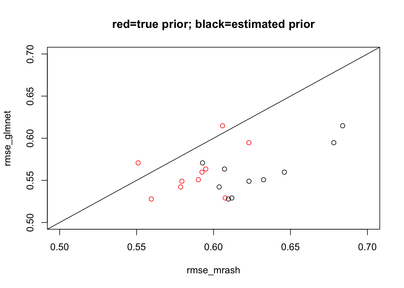
Attempt to find better initialization
Since the result is so consistently that mr.ash is worse than lasso here, I’ll initially just focus on the last of the simulations above.
The first thing I wanted to try was fixing the prior to the “true” value. I was suprised to find I actually needed to use the true beta to initialize in order to get good error. And the initialization really changes things, even with true fixed prior.
s2 = (sqrt((1-pve)/(pve))*sd(sim$Y))^2

fit_trueg <- mr.ash.alpha::mr.ash(sim$X, sim$Y,standardize = FALSE, sa2 = c(0,1/s2), pi=c(0.5,0.5), sigma2 = s2, update.pi=FALSE, update.sigma2 = FALSE, intercept=FALSE,min.iter=100)
Mr.ASH terminated at iteration 920.Warning in mr.ash.alpha::mr.ash(sim$X, sim$Y, standardize = FALSE, sa2 = c(0, :
The mixture proportion associated with the largest prior variance is greater
than zero; this indicates that the model fit could be improved by using a larger
setting of the prior variance. Consider increasing the range of the variances
"sa2".fit_trueg.inittrueb <- mr.ash.alpha::mr.ash(sim$X, sim$Y,standardize = FALSE, sa2 = c(0,1/s2), beta.init=sim$B, pi=c(0.5,0.5), sigma2 = s2, update.pi=FALSE, update.sigma2 = FALSE, intercept = FALSE)Mr.ASH terminated at iteration 422.Warning in mr.ash.alpha::mr.ash(sim$X, sim$Y, standardize = FALSE, sa2 = c(0, :
The mixture proportion associated with the largest prior variance is greater
than zero; this indicates that the model fit could be improved by using a larger
setting of the prior variance. Consider increasing the range of the variances
"sa2".sqrt(mean((sim$B-fit_trueg$beta)^2))[1] 0.5794779sqrt(mean((sim$B-fit_trueg.inittrueb$beta)^2))[1] 0.4648451plot(fit_trueg$beta, fit_trueg.inittrueb$beta)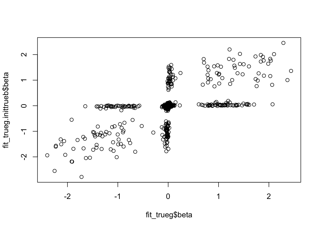
| Version | Author | Date |
|---|---|---|
| d7157a8 | Matthew Stephens | 2020-06-19 |
Reassuringly, the better solution also has better objective (but only slightly).
min(fit_trueg$varobj)[1] 2375.551min(fit_trueg.inittrueb$varobj)[1] 2385.549Try to initialize based on Lasso fit
Here I investigate some ideas to try to get the mr.ash prior to fit the lasso prior.
First I will compute the values of \(\tilde{b}\), which, algorithmically, are the values of \(b\) before shrinkage (soft-thresholding) is applied to them. I’m going to look at the shrinkage factors, which I define to be \(f:=b/\tilde{b}\).
y = sim$Y
X = sim$X
d = colSums(X^2)
b = coef(fit_glmnet)[-1]
r = y-sim$X %*% b - coef(fit_glmnet)[1]
btilde = drop((t(X) %*% r)/d) + b

plot(btilde,b, main="btilde vs b from lasso")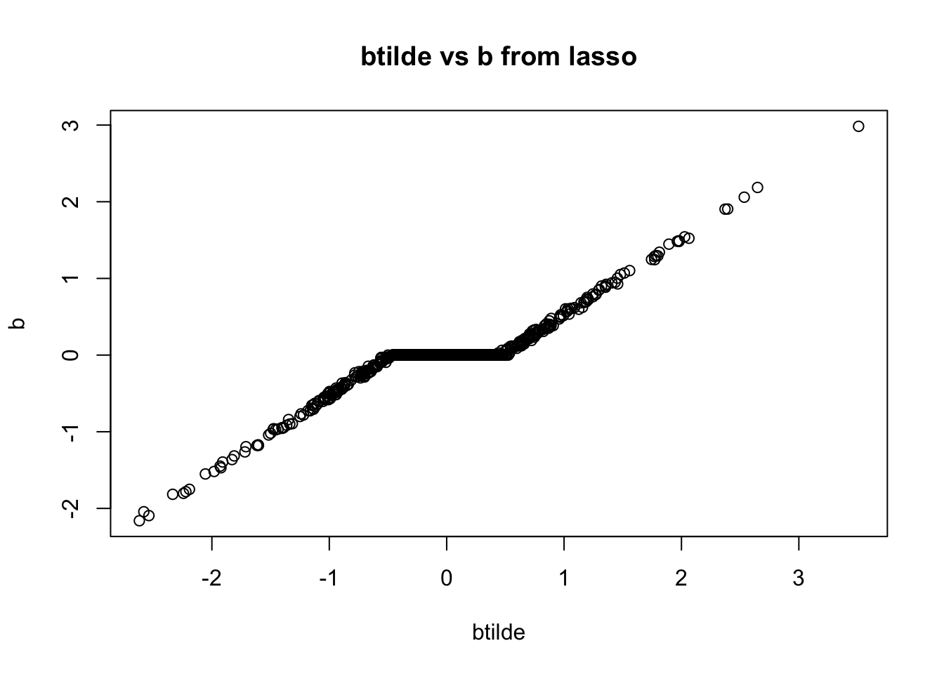
hist(b/btilde,nclass=100, main = "histogram of shrinkage factors from lasso fit")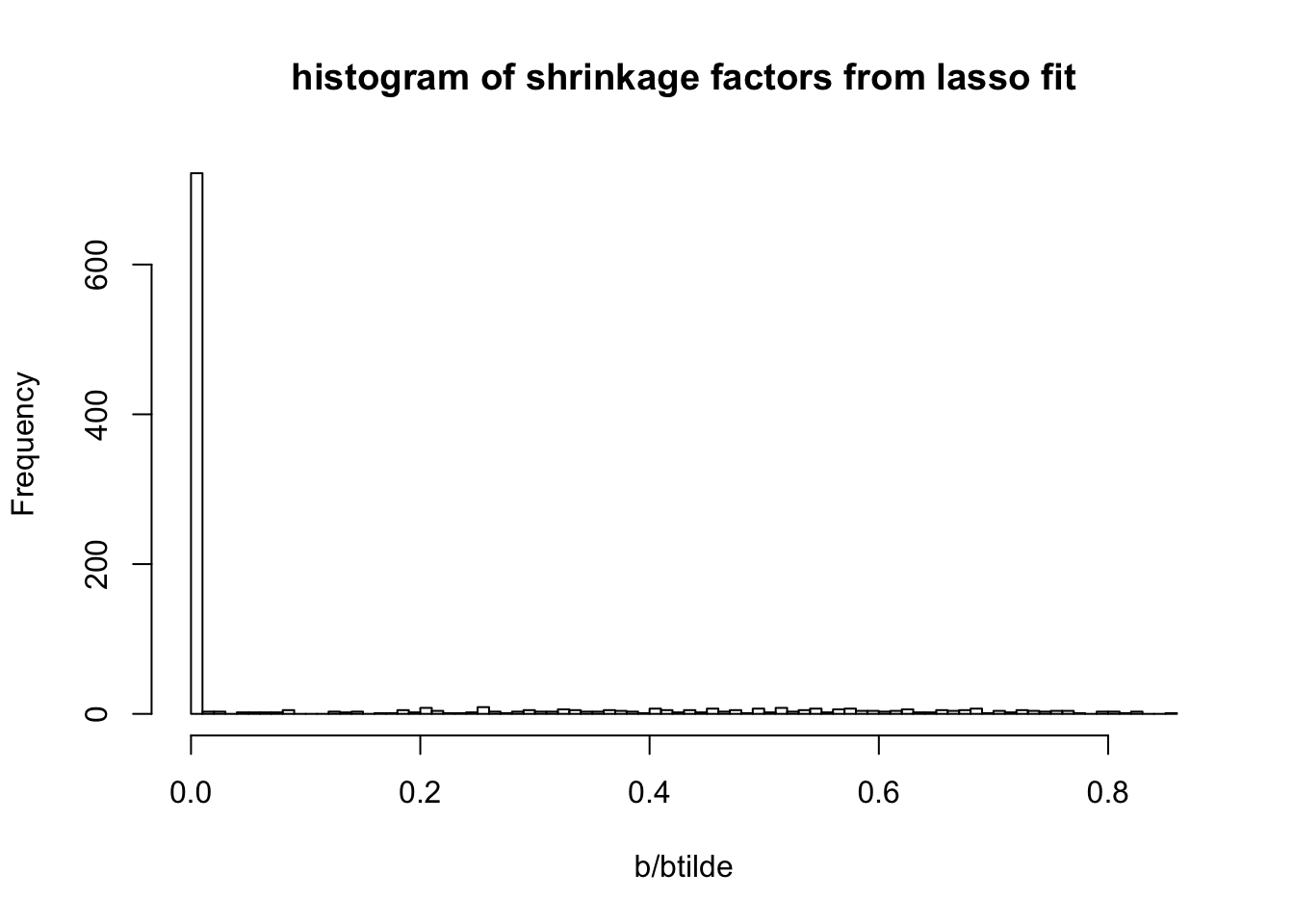
We want to try to select a prior such that the mr ash shrinkage operator is similar to the lasso. Intuitively that will ensure that the first mr ash update step does not change the solution “very much”. Ideally one might select \(g\) to minimize \(b-S_g(btilde)\).
THe mr ash shrinkage operator is the average of many ridge regression shrinkage operators. In ridge regression, with prior sa2 s2 the shrinkage factor for a variable \(j\) is \(f_j = sa2/(sa2 + 1/d_j)\), where \(d_j = x_j'x_j\).
Rearranging, and writing the shrinkage factor as \(f\), \((d sa2 + 1) f_j = d_j sa2\) or \[sa2 = f_j/[d_j(1-f)]\]
To get a quick approximation of what \(g\) might be we take the empirical values for sa2 computed in this way from the shrinkage factors. To give a grid I then cluster these empirical values into quantiles and give them equal weights in the prior. I deal separately with shrinkage factor 0.
f = b/btilde
sa2 = f/(d*(1-f))
hist(sa2)
| Version | Author | Date |
|---|---|---|
| d7157a8 | Matthew Stephens | 2020-06-19 |
pi0 = mean(sa2==0)
sa2 = sa2[sa2!=0] # deal with zeros separately

sa2 = as.vector(quantile(sa2,seq(0,1,length=20)))
sa2 = c(0,sa2)
w = c(pi0, (1-pi0)*rep(1/20,20))
Here I write code to compute posterior mean under normal means model with given prior variances and data variances. (Note the prior variances here not scaled by data variances.)
softmax = function(x){
    x = x- max(x)
    y = exp(x)
    return(y/sum(y))
}

postmean = function(b, w, prior_variances, data_variance){
  total_var = prior_variances + data_variance
  loglik = -0.5* log(total_var) + dnorm(outer(sqrt(1/total_var),b,FUN="*"),log=TRUE) # K by p matrix
  log_post = loglik + log(w)
  phi = apply(log_post, 2, softmax)
  mu = outer(prior_variances/total_var,b)
  return(colSums(phi*mu))
}
Now check if our prior reproduces the lasso shrinkage approximately. It does!
plot(btilde,b, main="comparison of mr.ash shrinkage (red) with soft thresholding")

lines(sort(btilde),postmean(sort(btilde), w, prior_variances = s2*sa2, data_variance = s2/median(d)),col=2,lwd=2)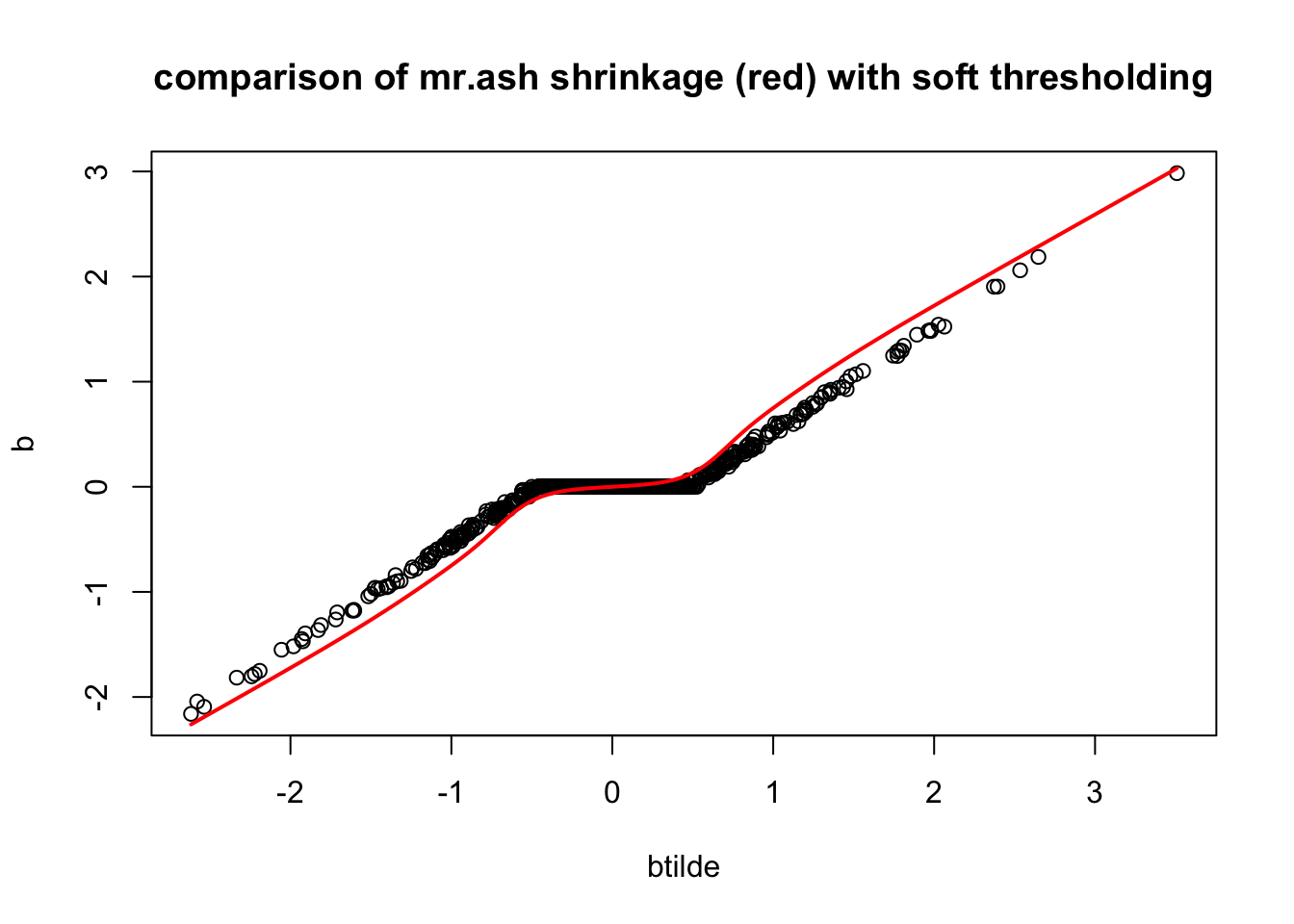
Somewhat unexpectedly though, initializing here has no effect
fit_mrash = mr.ash.alpha::mr.ash(sim$X, sim$Y,standardize = FALSE)Mr.ASH terminated at iteration 414.fit_mrash_lassoinit <- mr.ash.alpha::mr.ash(sim$X, sim$Y,standardize = FALSE, beta.init = b, sa2 = sa2, pi=w, sigma2=s2)Mr.ASH terminated at iteration 1000.Warning in mr.ash.alpha::mr.ash(sim$X, sim$Y, standardize = FALSE, beta.init
= b, : The mixture proportion associated with the largest prior variance is
greater than zero; this indicates that the model fit could be improved by using
a larger setting of the prior variance. Consider increasing the range of the
variances "sa2".plot(fit_mrash_lassoinit$beta,fit_mrash$beta)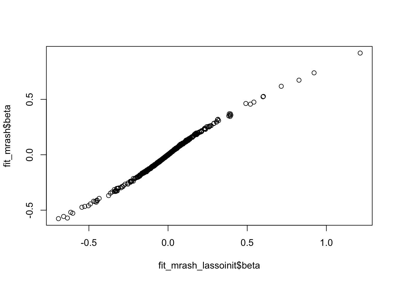
| Version | Author | Date |
|---|---|---|
| d7157a8 | Matthew Stephens | 2020-06-19 |
sqrt(mean((sim$B-fit_mrash_lassoinit$beta)^2))[1] 0.6073579sqrt(mean((sim$B-fit_mrash$beta)^2))[1] 0.6096696min(fit_mrash$varobj)[1] 2210.826min(fit_mrash_lassoinit$varobj)[1] 2210.982Plot the learned mr.mash shrinkage operators:
plot(btilde,b, main="comparison of mr.ash shrinkage (red) with soft thresholding")
lines(sort(btilde),postmean(sort(btilde), as.vector(fit_mrash$pi), prior_variances = fit_mrash$sigma2*fit_mrash$data$sa2, data_variance = fit_mrash$sigma2/median(d)),col=2,lwd=2)

lines(sort(btilde),postmean(sort(btilde), as.vector(fit_mrash_lassoinit$pi), prior_variances = fit_mrash_lassoinit$sigma2*fit_mrash_lassoinit$data$sa2, data_variance = fit_mrash_lassoinit$sigma2/median(d)),col=3,lwd=2)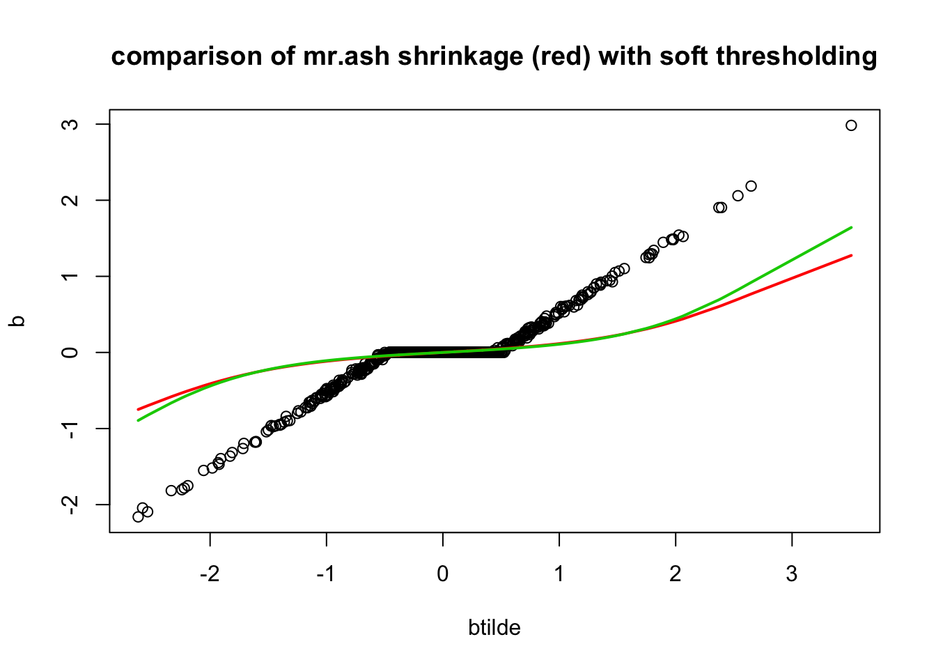
| Version | Author | Date |
|---|---|---|
| d7157a8 | Matthew Stephens | 2020-06-19 |
Interestingly the fitted pi from lasso initialization is almost identical to the one used in lasso. So actually the prior is the same! It is the sigma2 that must be different….
plot(fit_mrash_lassoinit$pi,w)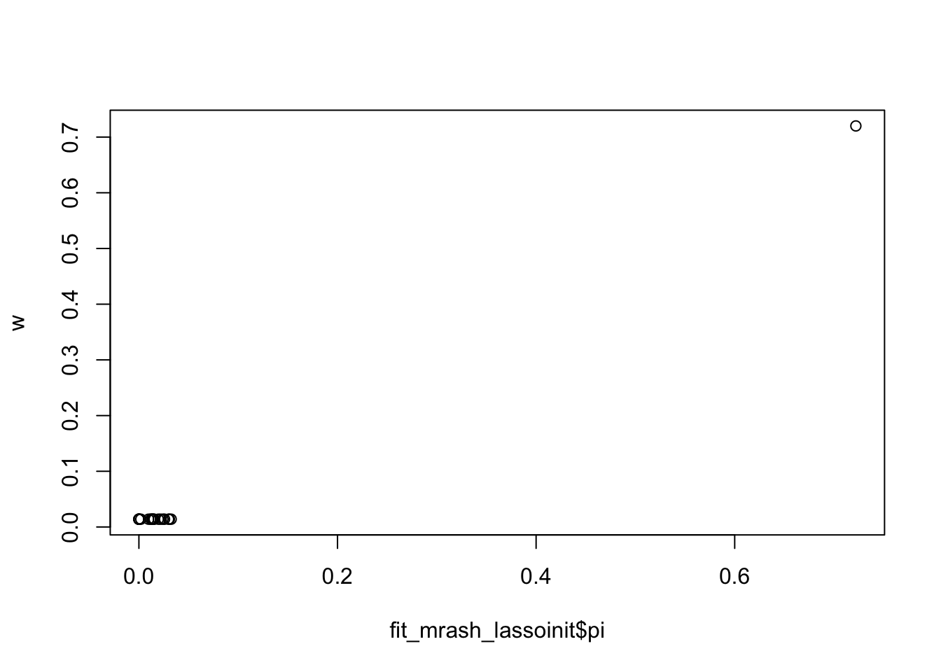
| Version | Author | Date |
|---|---|---|
| d7157a8 | Matthew Stephens | 2020-06-19 |
So here I fix sigma2:
fit_mrash_lassoinit_fixs2 <- mr.ash.alpha::mr.ash(sim$X, sim$Y,standardize = FALSE, beta.init = b, sa2 = sa2, pi=w, sigma2=s2, update.sigma2 = FALSE)Mr.ASH terminated at iteration 247.Warning in mr.ash.alpha::mr.ash(sim$X, sim$Y, standardize = FALSE, beta.init
= b, : The mixture proportion associated with the largest prior variance is
greater than zero; this indicates that the model fit could be improved by using
a larger setting of the prior variance. Consider increasing the range of the
variances "sa2".sqrt(mean((sim$B-fit_mrash_lassoinit_fixs2$beta)^2))[1] 0.4895231And now initialize from that fit:
fit_mrash_lassoinit_relaxs2 <- mr.ash.alpha::mr.ash(sim$X, sim$Y,standardize = FALSE, beta.init = fit_mrash_lassoinit_fixs2$beta, sa2 = fit_mrash_lassoinit_fixs2$data$sa2, pi=fit_mrash_lassoinit_fixs2$pi, sigma2=fit_mrash_lassoinit_fixs2$sigma2)Mr.ASH terminated at iteration 352.Warning in mr.ash.alpha::mr.ash(sim$X, sim$Y, standardize = FALSE, beta.init
= fit_mrash_lassoinit_fixs2$beta, : The mixture proportion associated with the
largest prior variance is greater than zero; this indicates that the model fit
could be improved by using a larger setting of the prior variance. Consider
increasing the range of the variances "sa2".sqrt(mean((sim$B-fit_mrash_lassoinit_relaxs2$beta)^2))[1] 0.5878811min(fit_mrash_lassoinit_relaxs2$varobj)[1] 2215.352min(fit_mrash_lassoinit_fixs2$varobj)[1] 2464.858Initializing from ridge regression
One of the challenges is that the mr ash shrinkage operator is not a special case of lasso. In contrast, the ridge shrinkage operator is a special case. So it is easier to initialize from that.
Here i wanted to try this.
fit_ridge <- cv.glmnet(x=sim$X, y=sim$Y, family="gaussian", alpha=0, standardize=FALSE)
b = coef(fit_ridge)[-1]
r = y-sim$X %*% b - coef(fit_ridge)[1]
btilde = drop((t(X) %*% r)/d) + b

plot(btilde,b, main="btilde vs b from ridge")
abline(a=0,b=1)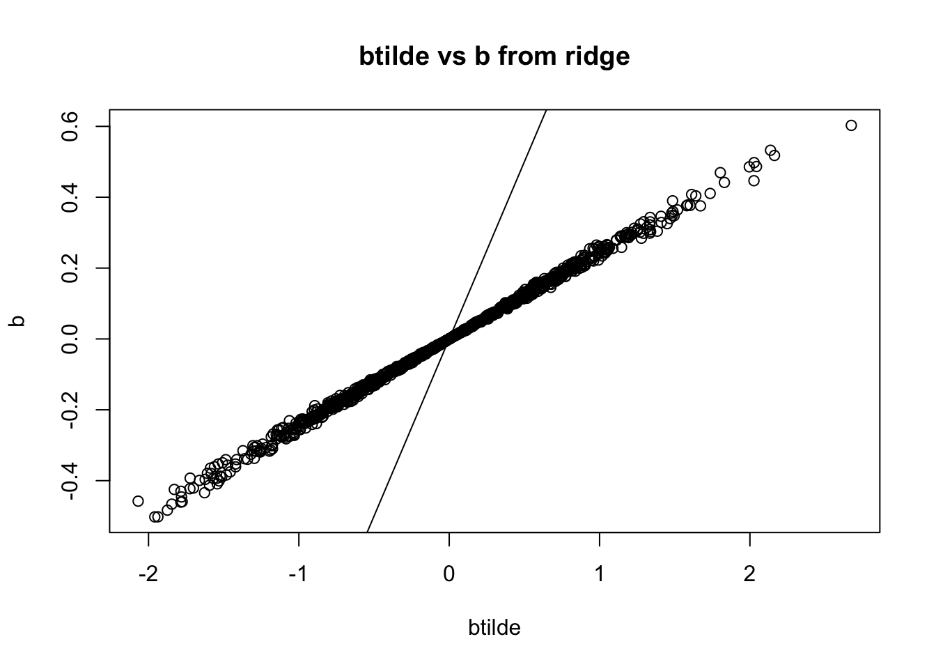
hist(b/btilde,nclass=100, main = "histogram of shrinkage factors from ridge fit")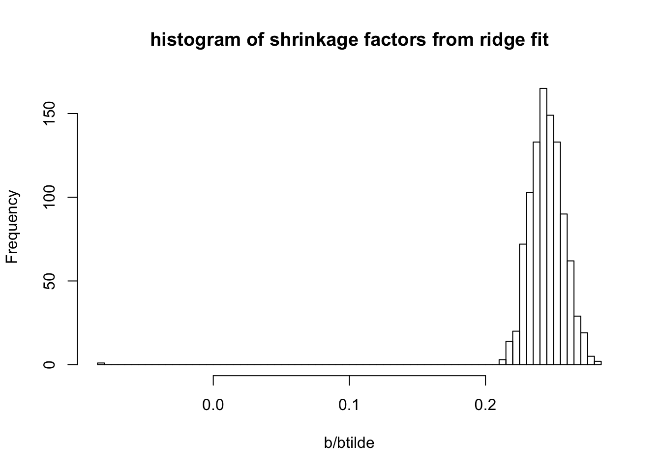
sqrt(mean((sim$B-b)^2))[1] 0.5908821
sessionInfo()R version 3.6.0 (2019-04-26)
Platform: x86_64-apple-darwin15.6.0 (64-bit)
Running under: macOS 10.16
Matrix products: default
BLAS: /Library/Frameworks/R.framework/Versions/3.6/Resources/lib/libRblas.0.dylib
LAPACK: /Library/Frameworks/R.framework/Versions/3.6/Resources/lib/libRlapack.dylib
locale:
[1] en_US.UTF-8/en_US.UTF-8/en_US.UTF-8/C/en_US.UTF-8/en_US.UTF-8
attached base packages:
[1] stats graphics grDevices utils datasets methods base
other attached packages:
[1] glmnet_4.1 Matrix_1.2-18 mr.ash.alpha_0.1-36
loaded via a namespace (and not attached):
[1] Rcpp_1.0.6 pillar_1.4.6 compiler_3.6.0 later_1.1.0.1
[5] git2r_0.27.1 workflowr_1.6.2 iterators_1.0.12 tools_3.6.0
[9] digest_0.6.27 evaluate_0.14 lifecycle_0.2.0 tibble_3.0.4
[13] lattice_0.20-41 pkgconfig_2.0.3 rlang_0.4.8 foreach_1.5.0
[17] rstudioapi_0.11 yaml_2.2.1 xfun_0.16 stringr_1.4.0
[21] knitr_1.29 fs_1.5.0 vctrs_0.3.4 rprojroot_1.3-2
[25] grid_3.6.0 glue_1.4.2 R6_2.4.1 survival_3.2-3
[29] rmarkdown_2.3 magrittr_1.5 whisker_0.4 splines_3.6.0
[33] backports_1.1.10 promises_1.1.1 codetools_0.2-16 ellipsis_0.3.1
[37] htmltools_0.5.0 shape_1.4.4 httpuv_1.5.4 stringi_1.4.6
[41] crayon_1.3.4