nmu_em

workflowr

• Summary
• Checks
• Past versions

Last updated: 2025-03-11

Checks: 7 0

Knit directory: misc/analysis/

This reproducible R Markdown analysis was created with workflowr (version 1.7.1). The Checks tab describes the reproducibility checks that were applied when the results were created. The Past versions tab lists the development history.

---

R Markdown file: up-to-date

Great! Since the R Markdown file has been committed to the Git repository, you know the exact version of the code that produced these results.

Environment: empty

Great job! The global environment was empty. Objects defined in the global environment can affect the analysis in your R Markdown file in unknown ways. For reproduciblity it’s best to always run the code in an empty environment.

Seed: set.seed(1)

The command set.seed(1) was run prior to running the code in the R Markdown file. Setting a seed ensures that any results that rely on randomness, e.g. subsampling or permutations, are reproducible.

Session information: recorded

Great job! Recording the operating system, R version, and package versions is critical for reproducibility.

Cache: none

Nice! There were no cached chunks for this analysis, so you can be confident that you successfully produced the results during this run.

File paths: relative

Great job! Using relative paths to the files within your workflowr project makes it easier to run your code on other machines.

Repository version: a4be13a

Great! You are using Git for version control. Tracking code development and connecting the code version to the results is critical for reproducibility.

The results in this page were generated with repository version a4be13a. See the Past versions tab to see a history of the changes made to the R Markdown and HTML files.

Note that you need to be careful to ensure that all relevant files for the analysis have been committed to Git prior to generating the results (you can use wflow_publish or wflow_git_commit). workflowr only checks the R Markdown file, but you know if there are other scripts or data files that it depends on. Below is the status of the Git repository when the results were generated:

Ignored files:
    Ignored:    .DS_Store
    Ignored:    .Rhistory
    Ignored:    .Rproj.user/
    Ignored:    analysis/.RData
    Ignored:    analysis/.Rhistory
    Ignored:    analysis/ALStruct_cache/
    Ignored:    data/.Rhistory
    Ignored:    data/methylation-data-for-matthew.rds
    Ignored:    data/pbmc/
    Ignored:    data/pbmc_purified.RData

Untracked files:
    Untracked:  .dropbox
    Untracked:  Icon
    Untracked:  analysis/GHstan.Rmd
    Untracked:  analysis/GTEX-cogaps.Rmd
    Untracked:  analysis/PACS.Rmd
    Untracked:  analysis/Rplot.png
    Untracked:  analysis/SPCAvRP.rmd
    Untracked:  analysis/abf_comparisons.Rmd
    Untracked:  analysis/admm_02.Rmd
    Untracked:  analysis/admm_03.Rmd
    Untracked:  analysis/bispca.Rmd
    Untracked:  analysis/cache/
    Untracked:  analysis/cholesky.Rmd
    Untracked:  analysis/compare-transformed-models.Rmd
    Untracked:  analysis/cormotif.Rmd
    Untracked:  analysis/cp_ash.Rmd
    Untracked:  analysis/eQTL.perm.rand.pdf
    Untracked:  analysis/eb_prepilot.Rmd
    Untracked:  analysis/eb_var.Rmd
    Untracked:  analysis/ebpmf1.Rmd
    Untracked:  analysis/ebpmf_sla_text.Rmd
    Untracked:  analysis/ebpower.Rmd
    Untracked:  analysis/ebspca_sims.Rmd
    Untracked:  analysis/explore_psvd.Rmd
    Untracked:  analysis/fa_check_identify.Rmd
    Untracked:  analysis/fa_iterative.Rmd
    Untracked:  analysis/flash_cov_overlapping_groups_init.Rmd
    Untracked:  analysis/flash_test_tree.Rmd
    Untracked:  analysis/flashier_newgroups.Rmd
    Untracked:  analysis/flashier_nmf_triples.Rmd
    Untracked:  analysis/flashier_pbmc.Rmd
    Untracked:  analysis/flashier_snn_shifted_prior.Rmd
    Untracked:  analysis/greedy_ebpmf_exploration_00.Rmd
    Untracked:  analysis/ieQTL.perm.rand.pdf
    Untracked:  analysis/lasso_em_03.Rmd
    Untracked:  analysis/m6amash.Rmd
    Untracked:  analysis/mash_bhat_z.Rmd
    Untracked:  analysis/mash_ieqtl_permutations.Rmd
    Untracked:  analysis/methylation_example.Rmd
    Untracked:  analysis/mixsqp.Rmd
    Untracked:  analysis/mr.ash_lasso_init.Rmd
    Untracked:  analysis/mr.mash.test.Rmd
    Untracked:  analysis/mr_ash_modular.Rmd
    Untracked:  analysis/mr_ash_parameterization.Rmd
    Untracked:  analysis/mr_ash_ridge.Rmd
    Untracked:  analysis/mv_gaussian_message_passing.Rmd
    Untracked:  analysis/nejm.Rmd
    Untracked:  analysis/nmf_bg.Rmd
    Untracked:  analysis/nonneg_underapprox.Rmd
    Untracked:  analysis/normal_conditional_on_r2.Rmd
    Untracked:  analysis/normalize.Rmd
    Untracked:  analysis/pbmc.Rmd
    Untracked:  analysis/pca_binary_weighted.Rmd
    Untracked:  analysis/pca_l1.Rmd
    Untracked:  analysis/poisson_nmf_approx.Rmd
    Untracked:  analysis/poisson_shrink.Rmd
    Untracked:  analysis/poisson_transform.Rmd
    Untracked:  analysis/qrnotes.txt
    Untracked:  analysis/ridge_iterative_02.Rmd
    Untracked:  analysis/ridge_iterative_splitting.Rmd
    Untracked:  analysis/samps/
    Untracked:  analysis/sc_bimodal.Rmd
    Untracked:  analysis/shrinkage_comparisons_changepoints.Rmd
    Untracked:  analysis/susie_cov.Rmd
    Untracked:  analysis/susie_en.Rmd
    Untracked:  analysis/susie_z_investigate.Rmd
    Untracked:  analysis/svd-timing.Rmd
    Untracked:  analysis/temp.RDS
    Untracked:  analysis/temp.Rmd
    Untracked:  analysis/test-figure/
    Untracked:  analysis/test.Rmd
    Untracked:  analysis/test.Rpres
    Untracked:  analysis/test.md
    Untracked:  analysis/test_qr.R
    Untracked:  analysis/test_sparse.Rmd
    Untracked:  analysis/tree_dist_top_eigenvector.Rmd
    Untracked:  analysis/z.txt
    Untracked:  code/multivariate_testfuncs.R
    Untracked:  code/rqb.hacked.R
    Untracked:  data/4matthew/
    Untracked:  data/4matthew2/
    Untracked:  data/E-MTAB-2805.processed.1/
    Untracked:  data/ENSG00000156738.Sim_Y2.RDS
    Untracked:  data/GDS5363_full.soft.gz
    Untracked:  data/GSE41265_allGenesTPM.txt
    Untracked:  data/Muscle_Skeletal.ACTN3.pm1Mb.RDS
    Untracked:  data/P.rds
    Untracked:  data/Thyroid.FMO2.pm1Mb.RDS
    Untracked:  data/bmass.HaemgenRBC2016.MAF01.Vs2.MergedDataSources.200kRanSubset.ChrBPMAFMarkerZScores.vs1.txt.gz
    Untracked:  data/bmass.HaemgenRBC2016.Vs2.NewSNPs.ZScores.hclust.vs1.txt
    Untracked:  data/bmass.HaemgenRBC2016.Vs2.PreviousSNPs.ZScores.hclust.vs1.txt
    Untracked:  data/eb_prepilot/
    Untracked:  data/finemap_data/fmo2.sim/b.txt
    Untracked:  data/finemap_data/fmo2.sim/dap_out.txt
    Untracked:  data/finemap_data/fmo2.sim/dap_out2.txt
    Untracked:  data/finemap_data/fmo2.sim/dap_out2_snp.txt
    Untracked:  data/finemap_data/fmo2.sim/dap_out_snp.txt
    Untracked:  data/finemap_data/fmo2.sim/data
    Untracked:  data/finemap_data/fmo2.sim/fmo2.sim.config
    Untracked:  data/finemap_data/fmo2.sim/fmo2.sim.k
    Untracked:  data/finemap_data/fmo2.sim/fmo2.sim.k4.config
    Untracked:  data/finemap_data/fmo2.sim/fmo2.sim.k4.snp
    Untracked:  data/finemap_data/fmo2.sim/fmo2.sim.ld
    Untracked:  data/finemap_data/fmo2.sim/fmo2.sim.snp
    Untracked:  data/finemap_data/fmo2.sim/fmo2.sim.z
    Untracked:  data/finemap_data/fmo2.sim/pos.txt
    Untracked:  data/logm.csv
    Untracked:  data/m.cd.RDS
    Untracked:  data/m.cdu.old.RDS
    Untracked:  data/m.new.cd.RDS
    Untracked:  data/m.old.cd.RDS
    Untracked:  data/mainbib.bib.old
    Untracked:  data/mat.csv
    Untracked:  data/mat.txt
    Untracked:  data/mat_new.csv
    Untracked:  data/matrix_lik.rds
    Untracked:  data/paintor_data/
    Untracked:  data/running_data_chris.csv
    Untracked:  data/running_data_matthew.csv
    Untracked:  data/temp.txt
    Untracked:  data/y.txt
    Untracked:  data/y_f.txt
    Untracked:  data/zscore_jointLCLs_m6AQTLs_susie_eQTLpruned.rds
    Untracked:  data/zscore_jointLCLs_random.rds
    Untracked:  explore_udi.R
    Untracked:  output/fit.k10.rds
    Untracked:  output/fit.nn.pbmc.purified.rds
    Untracked:  output/fit.nn.rds
    Untracked:  output/fit.nn.s.001.rds
    Untracked:  output/fit.nn.s.01.rds
    Untracked:  output/fit.nn.s.1.rds
    Untracked:  output/fit.nn.s.10.rds
    Untracked:  output/fit.snn.s.001.rds
    Untracked:  output/fit.snn.s.01.nninit.rds
    Untracked:  output/fit.snn.s.01.rds
    Untracked:  output/fit.varbvs.RDS
    Untracked:  output/fit2.nn.pbmc.purified.rds
    Untracked:  output/glmnet.fit.RDS
    Untracked:  output/snn07.txt
    Untracked:  output/snn34.txt
    Untracked:  output/test.bv.txt
    Untracked:  output/test.gamma.txt
    Untracked:  output/test.hyp.txt
    Untracked:  output/test.log.txt
    Untracked:  output/test.param.txt
    Untracked:  output/test2.bv.txt
    Untracked:  output/test2.gamma.txt
    Untracked:  output/test2.hyp.txt
    Untracked:  output/test2.log.txt
    Untracked:  output/test2.param.txt
    Untracked:  output/test3.bv.txt
    Untracked:  output/test3.gamma.txt
    Untracked:  output/test3.hyp.txt
    Untracked:  output/test3.log.txt
    Untracked:  output/test3.param.txt
    Untracked:  output/test4.bv.txt
    Untracked:  output/test4.gamma.txt
    Untracked:  output/test4.hyp.txt
    Untracked:  output/test4.log.txt
    Untracked:  output/test4.param.txt
    Untracked:  output/test5.bv.txt
    Untracked:  output/test5.gamma.txt
    Untracked:  output/test5.hyp.txt
    Untracked:  output/test5.log.txt
    Untracked:  output/test5.param.txt

Unstaged changes:
    Modified:   .gitignore
    Modified:   analysis/flashier_log1p.Rmd
    Modified:   analysis/flashier_sla_text.Rmd
    Modified:   analysis/logistic_z_scores.Rmd
    Modified:   analysis/mr_ash_pen.Rmd
    Modified:   analysis/susie_flash.Rmd

Note that any generated files, e.g. HTML, png, CSS, etc., are not included in this status report because it is ok for generated content to have uncommitted changes.

---

These are the previous versions of the repository in which changes were made to the R Markdown (analysis/nmu_em.Rmd) and HTML (docs/nmu_em.html) files. If you’ve configured a remote Git repository (see ?wflow_git_remote), click on the hyperlinks in the table below to view the files as they were in that past version.

File	Version	Author	Date	Message
Rmd	a4be13a	Matthew Stephens	2025-03-11	workflowr::wflow_publish("nmu_em.Rmd")
html	8ac1380	Matthew Stephens	2025-02-27	Build site.
Rmd	f82707c	Matthew Stephens	2025-02-27	workflowr::wflow_publish("nmu_em.Rmd")
html	eb0b82b	Matthew Stephens	2025-02-26	Build site.
Rmd	19e41fe	Matthew Stephens	2025-02-26	wflow_publish("nmu_em.Rmd")

---

library("emg")

Loading required package: stats4

Loading required package: moments

library("tictoc")

Introduction

My goal is to fit a version of the non-negative matrix underapproximation using an EM algorithm.

The model for a data matrix \(A\) is: \[A = uv' + b + e\] where \(b_{ij} \sim Exp(\lambda)\), \(e_{ij} \sim N(0,sigma^2)\), and \(u,v\) are non-negative vectors to be estimated. Alternatively we could write \(A \sim N(uv' + b,\sigma^2)\). (Note: the distribution of the sum of independent exponential and gaussian random variables (\(b+e\)) is known as an exponentially modified gaussian (EMG) distribution. The emg package can be used to compute the density.)

If \(\sigma^2=0\) then the mle for \(u,v\) (integrating out \(b,e\)) should be a feasible solution to the underapproximation problem. However, introducing \(\sigma>0\) is useful because it allows us to implement an EM algorithm. If \(sigma^2\) is very small (compared with \(1/\lambda\)) then this will approximately solve (a version of) the non-negative matrix underapproximation problem. On the other hand, if \(1/\lambda\) is very small compared with \(\sigma\) then it will be closer to regular NMF.

NOTE: We could potentially use this idea within flashier to put priors on \(u\) and \(v\). Also, for modelling a symmetric matrix \(A\) we could instead fit \(A \sim N(uu'+b, \sigma^2)\).

The ELBO is \[F(u,v,q)= E_q((-1/2\sigma^2)||A-uv'-b||_2^2) + D_{KL}(q,g)\] where \(g\) is the prior on \(b\), \[g(b)=\lambda \exp(-\lambda b).\] Here \(q\) plays the role of the (approximate) posterior distribution on \(b\).

Given \(q\), the ELBO is minimized for \(u,v\) by solving \[\min_{u,v} ||A-\bar{b} - uv'||_2^2.\] Alternatively, any step that reduces this objective function will increase the ELBO. Here we will apply the truncated power method to achieve this.

Given \(u,v\) the ELBO is minimized by for each \(b_{ij}\) by solving \[q(b) \propto g(b) \exp((-1/2\sigma^2)(x_{ij}-b)^2) \propto \exp((-1/2\sigma^2)[b^2-2(x_{ij}-\lambda \sigma^2)b])\] where \(x_{ij} = A_ij - u_i v_j\). This is a truncated normal distribution, \[ q(b_{ij}) = N_+(x_{ij}-\lambda \sigma^2, \sigma^2)\]. Fortunately, the mean of this distribution is easily computed.

Note: if \(\sigma\) is very small then the mean of this truncated normal looks close to \((x)_+\).

  sigma=0.01  
  x = seq(-0.5,0.5,length=20)
  plot(x,truncnorm::etruncnorm(0,Inf,x-sigma^2,sigma))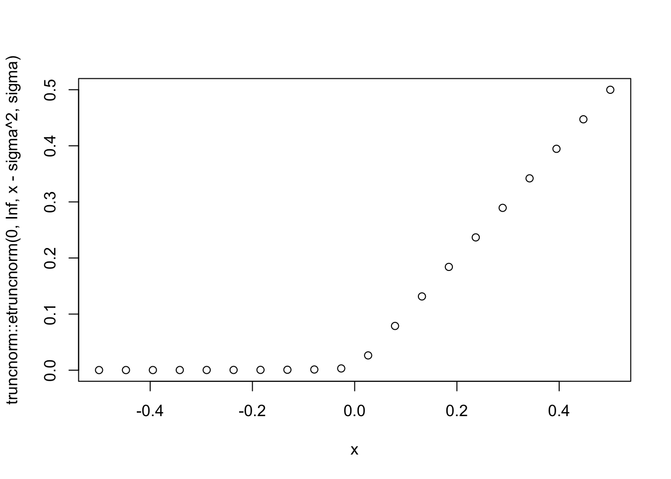

Past versions of unnamed-chunk-2-1.png

Version	Author	Date
8ac1380	Matthew Stephens	2025-02-27

Implementation (symmetric A)

I’m going to try the symmetric case (\(A\) symmetric; \(u=v\)). First I simulate some non-negative data for testing. A is a block covariance matrix of 0s and 1s plus non-negative noise.

set.seed(1)
n = 10
maxiter = 1000
x = cbind(c(rep(1,n),rep(0,n)), c(rep(0,n),rep(1,n)))
E = matrix(0.1*rexp(2*n*2*n),nrow=2*n)
E = E+t(E) #symmetric errors
A = x %*% t(x) + E
image(A)

Past versions of unnamed-chunk-3-1.png

Version	Author	Date
8ac1380	Matthew Stephens	2025-02-27
eb0b82b	Matthew Stephens	2025-02-26

I’m going to solve the symmetric nmf method by the thresholded power iteration, \[u \leftarrow (Au)_+\] Note: this is not an algorithm I can find a reference for but I believe it is true that, on rescaling u to have unit norm, this iteration decreases \(||A-uu'||\) subject to \(u>0\) \(||u||=1\). Then you can set \(d=u'Au\) to minimize \(||A-duu'||^2\).

#truncate and normalize function
trunc_and_norm = function(u){
  uplus = ifelse(u>0,u,0)
  if(!all(uplus==0))
    uplus = uplus/sqrt(sum(uplus^2))
  return(uplus)
}

loglik_emg = function(A,u,d,lambda,sigma){
  R = A- d * u %*% t(u)
  sum(demg(R,lambda=lambda,sigma=sigma,log=TRUE))
}

nmu_em = function(A, lambda=1, sigma=1, maxiter=100){
  b = matrix(0,nrow=nrow(A),ncol=ncol(A))

  # initialize u by svd (check both u and -u since either could work)
  u = svd(A)$u[,1]
  u1 = trunc_and_norm(u)
  u2 = trunc_and_norm(-u)
  if(t(u1) %*% A %*% u1 > t(u2) %*% A %*% u2){
    u = u1
  } else {
    u = u2
  }

  d = drop(t(u) %*% (A-b) %*% u)
  loglik = loglik_emg(A,u,d,lambda,sigma)
  
  for(i in 1:maxiter){
    u = trunc_and_norm((A-b) %*% u)
    d = drop(t(u) %*% (A-b) %*% u)
    b = matrix(truncnorm::etruncnorm(a=0,mean= A-d*u %*% t(u)-lambda*sigma^2,sd=sigma),nrow=2*n)
    loglik = c(loglik,loglik_emg(A,u,d,lambda,sigma))
  }

  d = drop(t(u) %*% (A-b) %*% u)
  return(list(u=u, d=d, b=b, loglik = loglik))
}

fit = nmu_em(A, 1, 1)
image(fit$u %*% t(fit$u))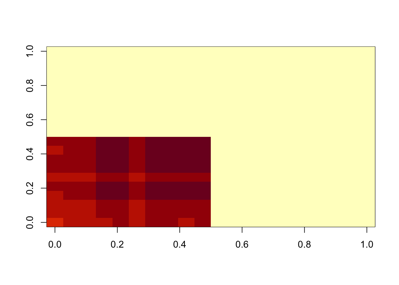

Past versions of unnamed-chunk-5-1.png

Version	Author	Date
8ac1380	Matthew Stephens	2025-02-27
eb0b82b	Matthew Stephens	2025-02-26

min(A- fit$d * fit$u %*% t(fit$u))

[1] 0.008737816

hist(A- fit$d * fit$u %*% t(fit$u))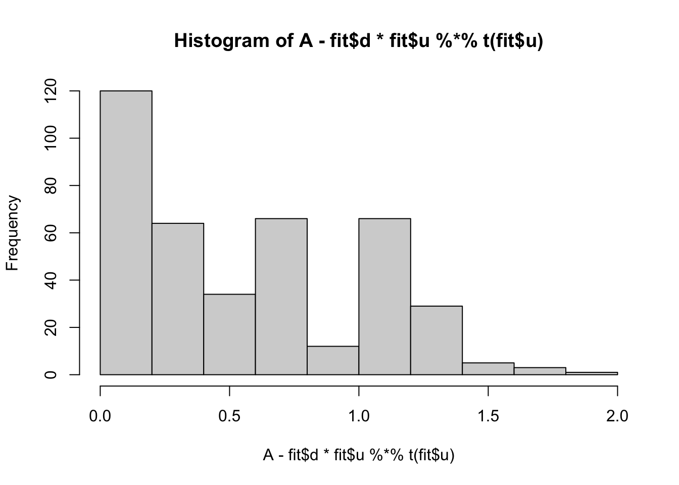

Past versions of unnamed-chunk-5-2.png

Version	Author	Date
8ac1380	Matthew Stephens	2025-02-27

plot(fit$loglik[-1])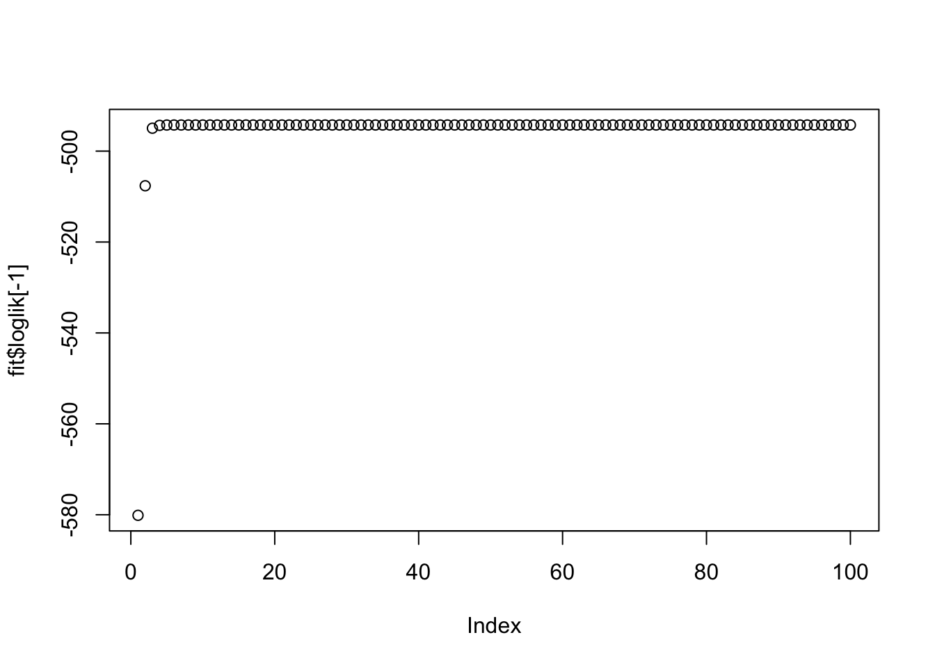

fit = nmu_em(A, 1, 0.1)
image(fit$u %*% t(fit$u))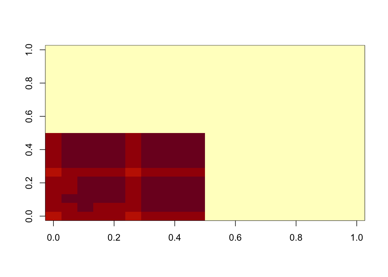

Past versions of unnamed-chunk-6-1.png

Version	Author	Date
8ac1380	Matthew Stephens	2025-02-27

min(A- fit$d * fit$u %*% t(fit$u))

[1] 0.008737816

hist(A- fit$d * fit$u %*% t(fit$u))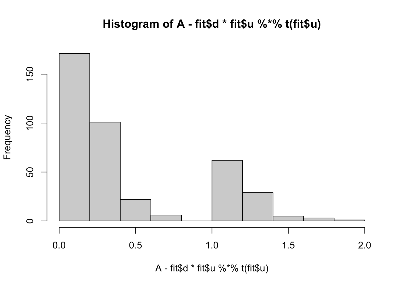

Past versions of unnamed-chunk-6-2.png

Version	Author	Date
8ac1380	Matthew Stephens	2025-02-27

plot(fit$loglik[-1])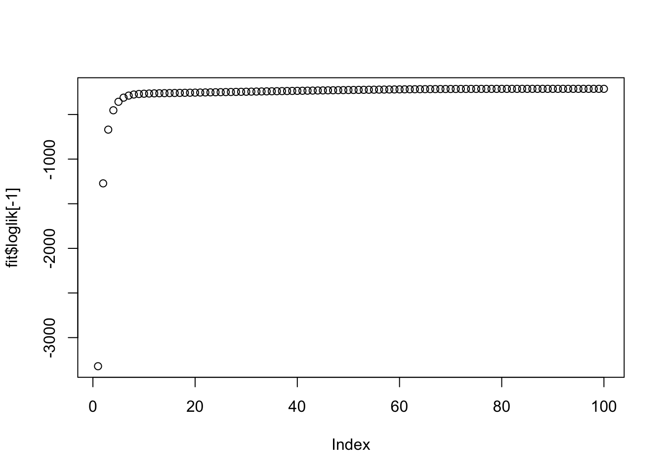

Note: if lambda is too small then the fit gets absorbed into b instead of u. This makes sense.

fit = nmu_em(A, .1, 1)
image(fit$u %*% t(fit$u))

Past versions of unnamed-chunk-7-1.png

Version	Author	Date
8ac1380	Matthew Stephens	2025-02-27
eb0b82b	Matthew Stephens	2025-02-26

image(fit$b)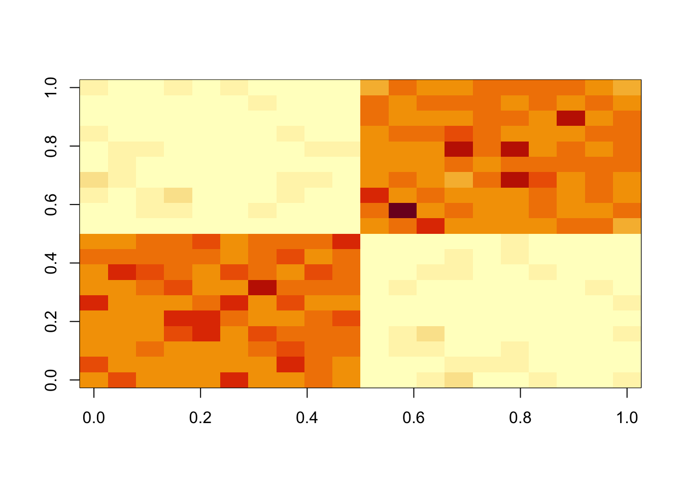

Past versions of unnamed-chunk-7-2.png

Version	Author	Date
8ac1380	Matthew Stephens	2025-02-27

More generally, if lambda and sigma are not appropriate this is unlikely to work well (note that the log-likelihood is not strictly increasing here, but is stable to 3dp so it is possible this is just numerical error rather than a bug.)

fit = nmu_em(A, 100, 100)
image(fit$u %*% t(fit$u))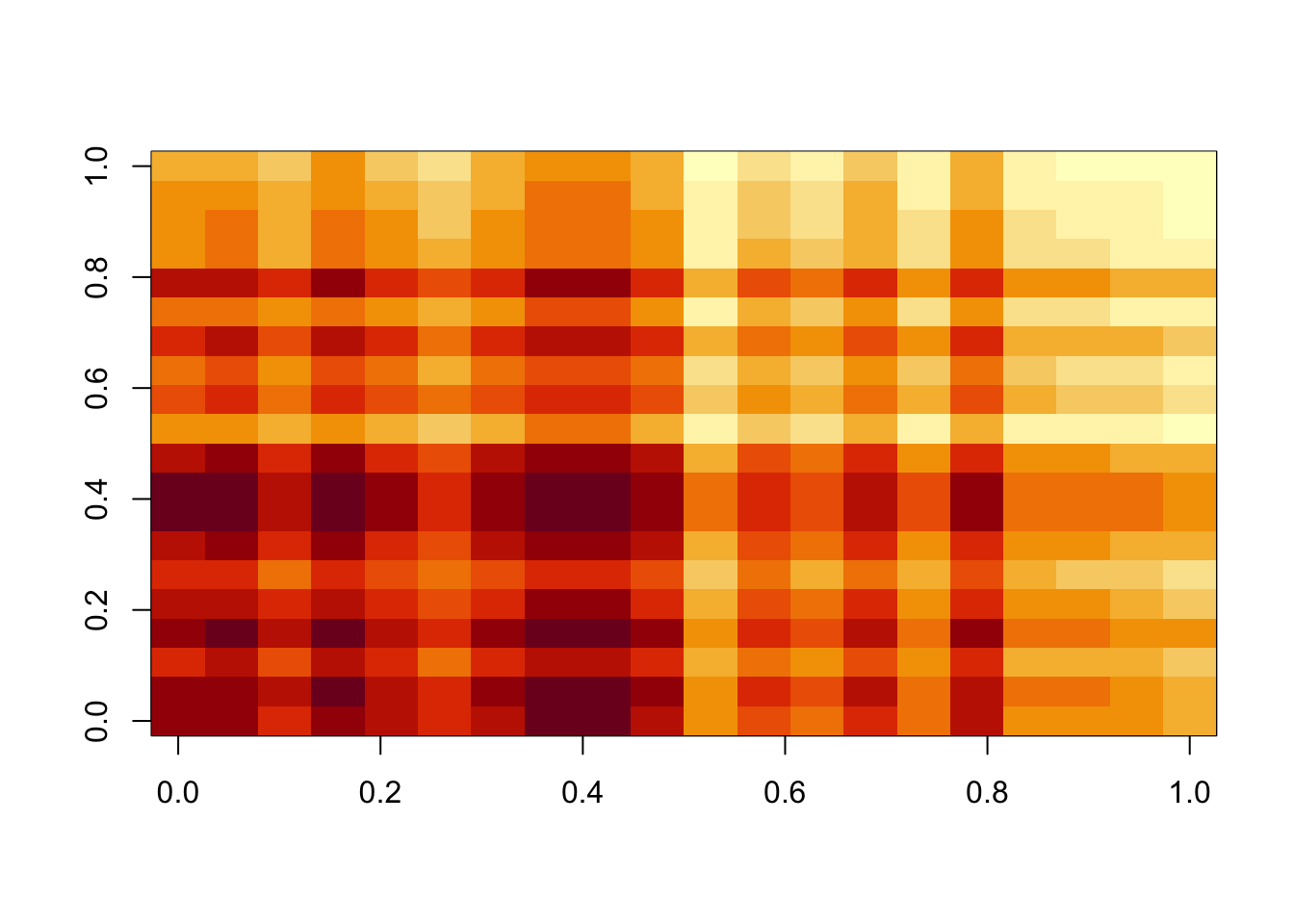

image(A-fit$d*fit$u %*% t(fit$u))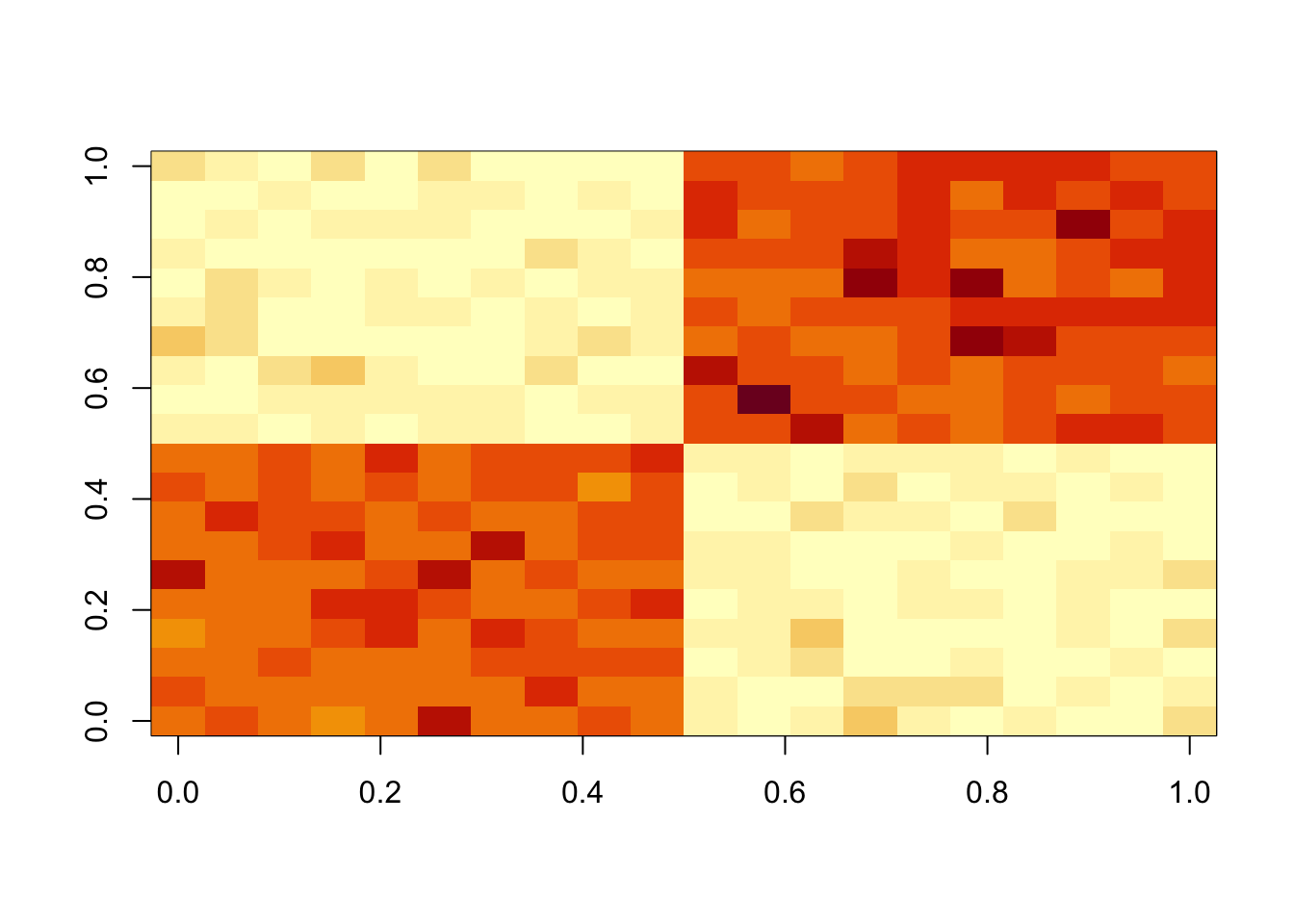

image(fit$b)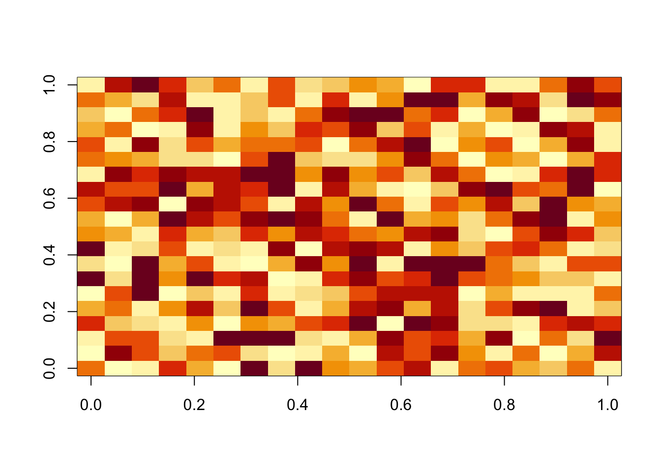

plot(fit$loglik)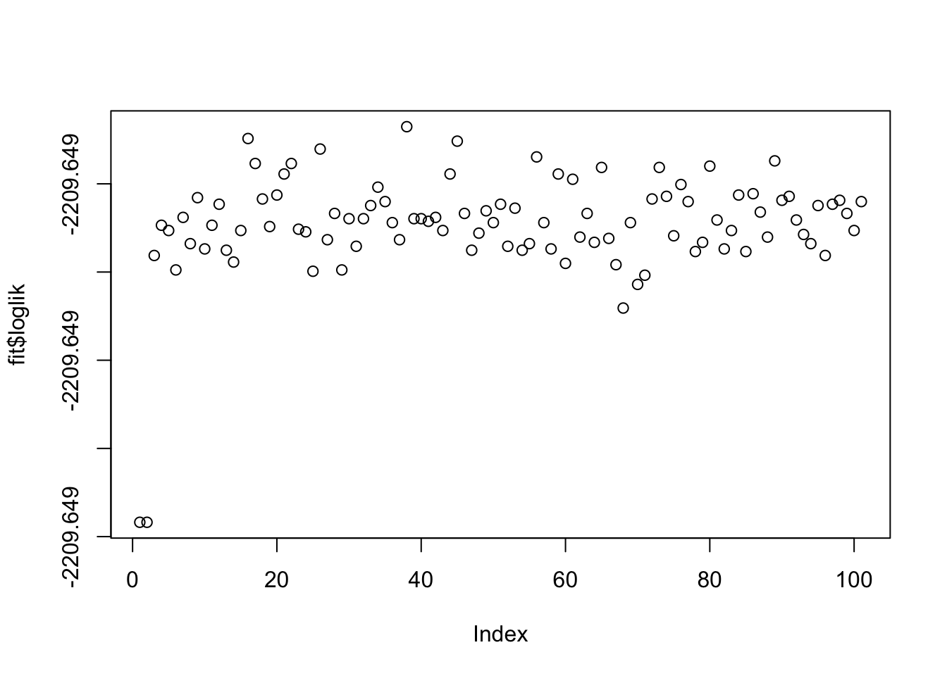

fit$loglik

  [1] -2209.649 -2209.649 -2209.649 -2209.649 -2209.649 -2209.649 -2209.649
  [8] -2209.649 -2209.649 -2209.649 -2209.649 -2209.649 -2209.649 -2209.649
 [15] -2209.649 -2209.649 -2209.649 -2209.649 -2209.649 -2209.649 -2209.649
 [22] -2209.649 -2209.649 -2209.649 -2209.649 -2209.649 -2209.649 -2209.649
 [29] -2209.649 -2209.649 -2209.649 -2209.649 -2209.649 -2209.649 -2209.649
 [36] -2209.649 -2209.649 -2209.649 -2209.649 -2209.649 -2209.649 -2209.649
 [43] -2209.649 -2209.649 -2209.649 -2209.649 -2209.649 -2209.649 -2209.649
 [50] -2209.649 -2209.649 -2209.649 -2209.649 -2209.649 -2209.649 -2209.649
 [57] -2209.649 -2209.649 -2209.649 -2209.649 -2209.649 -2209.649 -2209.649
 [64] -2209.649 -2209.649 -2209.649 -2209.649 -2209.649 -2209.649 -2209.649
 [71] -2209.649 -2209.649 -2209.649 -2209.649 -2209.649 -2209.649 -2209.649
 [78] -2209.649 -2209.649 -2209.649 -2209.649 -2209.649 -2209.649 -2209.649
 [85] -2209.649 -2209.649 -2209.649 -2209.649 -2209.649 -2209.649 -2209.649
 [92] -2209.649 -2209.649 -2209.649 -2209.649 -2209.649 -2209.649 -2209.649
 [99] -2209.649 -2209.649 -2209.649

Note: i did try applying this, accidentally, to a matrix where some A were negative, so there is no underapproximation solution. It still did something sensible, effectively trying to avoid reducing the negative entries any further. This is a nice feature.

Estimating lambda and sigma

I consider three possibilies. The first is a method of moments that is very simple.

Note that \[E(A-uv') = 1/\lambda\] and \[E(A-uv')^2 = 1/\lambda^2 + \sigma^2\]. So the method of moments gives \(\lambda = 1/mean(A-uv')\) and \(\sigma^2 = mean((A-uv')^2) - mean(A-uv')^2 = var(A-uv')\).

The second is maximum likelihood estimation of both lambda and sigma, done numerically.

The third is to estimate lambda by method of moments, and numerically optimize over sigma (I tried this because very preliminary results suggested that the MoM estimate for lambda may be more stable than that for sigma.)

The following code implements this idea (repeats estimating lambda,sigma up to 5 times). Note that this is really just an initial try. In practice, if we want an underapproximation, we might want to do something to ensure that sigma is small. Here I just initialize sigma to be small, but we need to think more about this, especially since we would like the method to be invariant to scaling of \(A\).

One possibility would be to initialize sigma to be the estimate based on the first PC, sigma= sqrt(mean((A - A.svd$d[1] * u %*% t(u))^2))
but maybe that is still too big since what we really want is that sigma is the residual when all of the (nonnegative) factors are taken out. Another possibility is to fix sigma by guessing that, say, the nonnegative factors will, in total, explain 99% of the variance.

#return the difference between the last and next-to-last elements of x
delta = function(x){
  return(x[length(x)]- x[length(x)-1])
}

nmu_em_estlambda = function(A, maxiter=100, lambda=1, sigma=0.1, est.method="mle.sigma", b.init = matrix(0,nrow=nrow(A),ncol=ncol(A))){

  b = b.init
  
  # if b.init supplied, use it to estimate lambda and sigma
  # this maybe only makes sense if we use the low rank approx of A to estimate b
  if(!missing(b.init)){ 
    lambda = 1/mean(b)
    sigma = sqrt(mean((A-b)^2))
  }  
    
  # initialize u by svd (check both u and -u since either could work)
  A.svd = svd(A)
  u = A.svd$u[,1]
  
  u1 = trunc_and_norm(u)
  u2 = trunc_and_norm(-u)
  if(t(u1) %*% A %*% u1 > t(u2) %*% A %*% u2){
    u = u1
  } else {
    u = u2
  }

  d = drop(t(u) %*% (A-b) %*% u)
  b = matrix(truncnorm::etruncnorm(a=0,mean= A-d*u %*% t(u)-lambda*sigma^2,sd=sigma),nrow=2*n)
  
  loglik = loglik_emg(A,u,d,lambda,sigma)
  
  for(j in 1:5){
    for(i in 1:maxiter){
      u = trunc_and_norm((A-b) %*% u)
      d = drop(t(u) %*% (A-b) %*% u)
      b = matrix(truncnorm::etruncnorm(a=0,mean= A-d*u %*% t(u)-lambda*sigma^2,sd=sigma),nrow=2*n)
      loglik = c(loglik, loglik_emg(A,u,d,lambda,sigma))
      if(delta(loglik)<1e-3) break;
    } 
    lambda = 1/mean(A-d * u %*% t(u)) #method of moments estimates
    sigma = sd(A-d * u %*% t(u))
    if(est.method == "mle.both"){
      fit.mle = mle(function(llambda,lsigma) {
          -loglik_emg(A, u, d, exp(llambda),exp(lsigma))
      }, method = "L-BFGS-B",lower = c(-10,-10), start =c(log(lambda),log(sigma)))
      lambda = exp(coef(fit.mle)[1])
      sigma = exp(coef(fit.mle)[2])
    }
    if(est.method == "mle.sigma"){
      fit.mle = mle(function(lsigma) {
          -loglik_emg(A, u, d, lambda,exp(lsigma))
      }, method = "Brent", lower=c(-10), upper = c(10), start =c(log(sigma)))
      sigma = exp(coef(fit.mle)[1])
    }
    
    loglik = c(loglik, loglik_emg(A,u,d,lambda,sigma))
    if(delta(loglik)<1e-3) break;
  }
  d = drop(t(u) %*% (A-b) %*% u)
  return(list(u=u, d=d, b=b, lambda=lambda, sigma=sigma, loglik = loglik))
}

Try it out. Note that MoM estimation of lambda, sigma decreases the loglikelihood.

set.seed(1)
n = 10
maxiter = 1000
x = cbind(c(rep(1,n),rep(0,n)), c(rep(0,n),rep(1,n)))
E = matrix(0.1*rexp(2*n*2*n),nrow=2*n)
E = E+t(E) #symmetric errors
A = x %*% t(x) + E
image(A)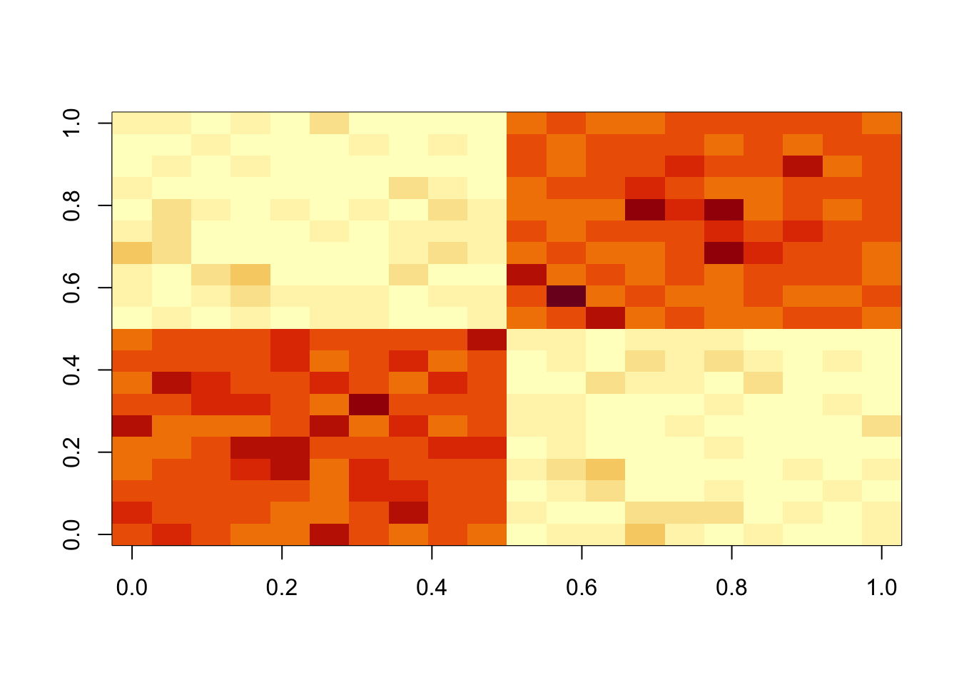

Past versions of unnamed-chunk-10-1.png

Version	Author	Date
8ac1380	Matthew Stephens	2025-02-27
eb0b82b	Matthew Stephens	2025-02-26

fit.mom = nmu_em_estlambda(A,est.method="mom")
fit.mle.both = nmu_em_estlambda(A,est.method="mle.both")
fit.mle.sigma = nmu_em_estlambda(A,est.method="mle.sigma")

fit.mom$lambda

[1] 2.220807

fit.mom$sigma

[1] 0.447544

fit.mle.both$lambda

 llambda 
2.235999 

fit.mle.both$sigma

     lsigma 
0.001436343 

fit.mle.sigma$lambda

[1] 2.235889

fit.mle.sigma$sigma

    lsigma 
0.00144136 

Note that estimates of lambda,sigma from mle.both and mle.sigma are almost identical. Also although estimates for lambda, sigma vary with mom, the estimated u is very similar.

plot(fit.mom$u)
points(fit.mle.both$u,col=2,pch=2)
points(fit.mle.sigma$u,col=3,pch=".")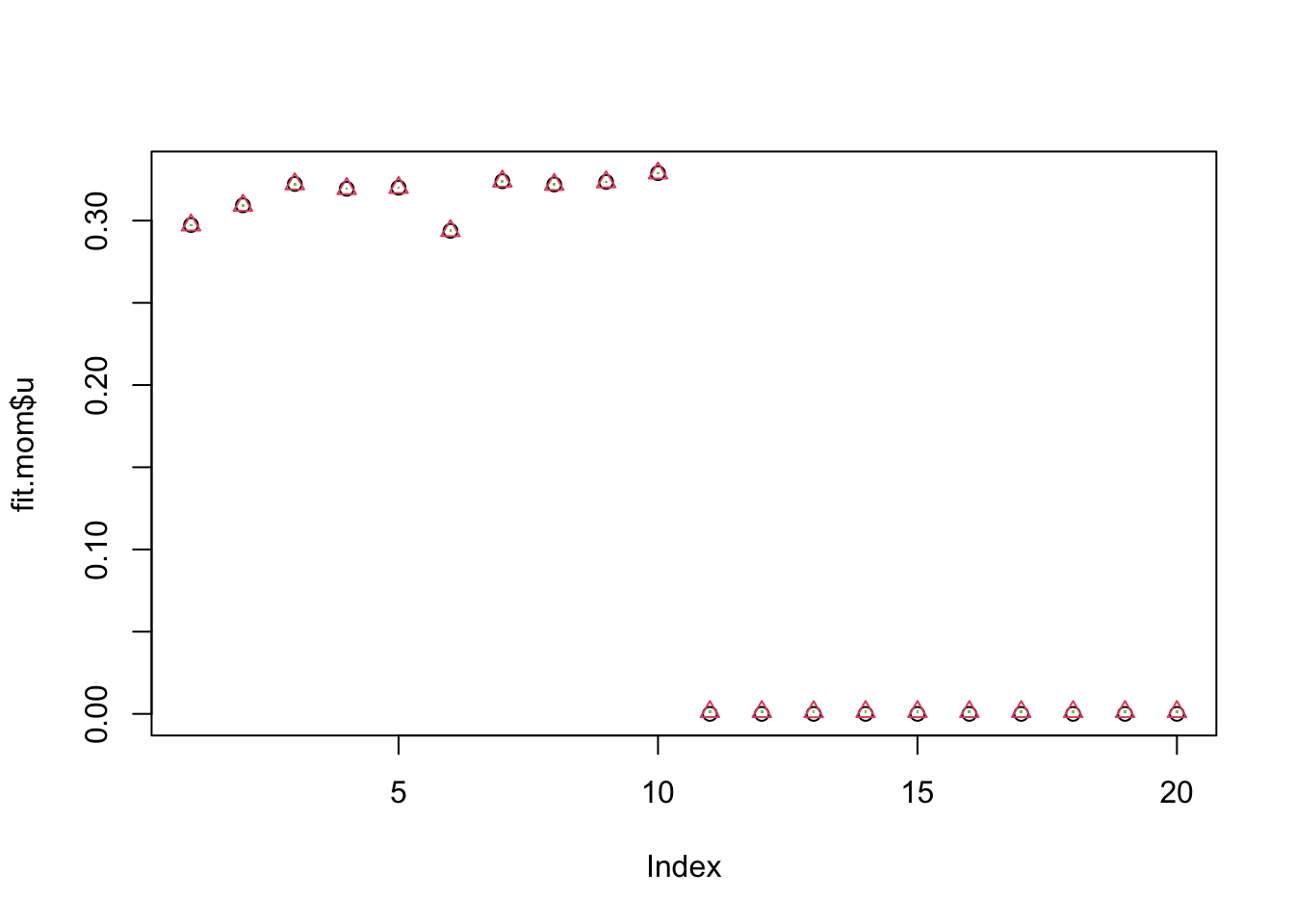

Past versions of unnamed-chunk-11-1.png

Version	Author	Date
8ac1380	Matthew Stephens	2025-02-27
eb0b82b	Matthew Stephens	2025-02-26

plot(fit.mle.both$loglik,col=2)
points(fit.mom$loglik)
points(fit.mle.sigma$loglik,col=3,pch=".")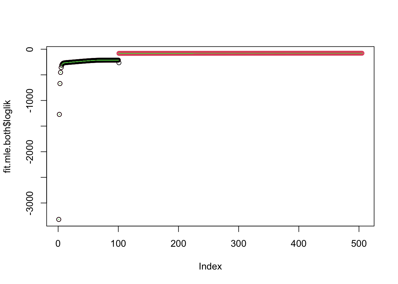

Past versions of unnamed-chunk-11-2.png

Version	Author	Date
8ac1380	Matthew Stephens	2025-02-27
eb0b82b	Matthew Stephens	2025-02-26

A tree

Try a tree, and iteratively removing factors. We can see this gives something close to the result we want. One question is why this happens because there seems to be a “better” solution even with underapproximation: I believe you can fit this tree with only four factors. This needs more investigation.

set.seed(1)
n = 40
x = cbind(c(rep(1,n),rep(0,n)), c(rep(0,n),rep(1,n)), c(rep(1,n/2),rep(0,3*n/2)), c(rep(0,n/2), rep(1,n/2), rep(0,n)), c(rep(0,n),rep(1,n/2),rep(0,n/2)), c(rep(0,3*n/2),rep(1,n/2)))
E = matrix(0.1*rexp(2*n*2*n),nrow=2*n)
E = E+t(E) #symmetric errors
A = x %*% t(x) + E

Method of moments:

A = x %*% t(x) + E
par(mfcol=c(3,3),mai=rep(0.2,4))
image(A)
tic()
for(i in 1:8){
  fit = nmu_em_estlambda(A,est.method = "mom")
  A = A-fit$d*fit$u %*% t(fit$u)
  fit$lambda
  fit$sigma
  plot(fit$u)
}

Past versions of unnamed-chunk-13-1.png

Version	Author	Date
8ac1380	Matthew Stephens	2025-02-27
eb0b82b	Matthew Stephens	2025-02-26

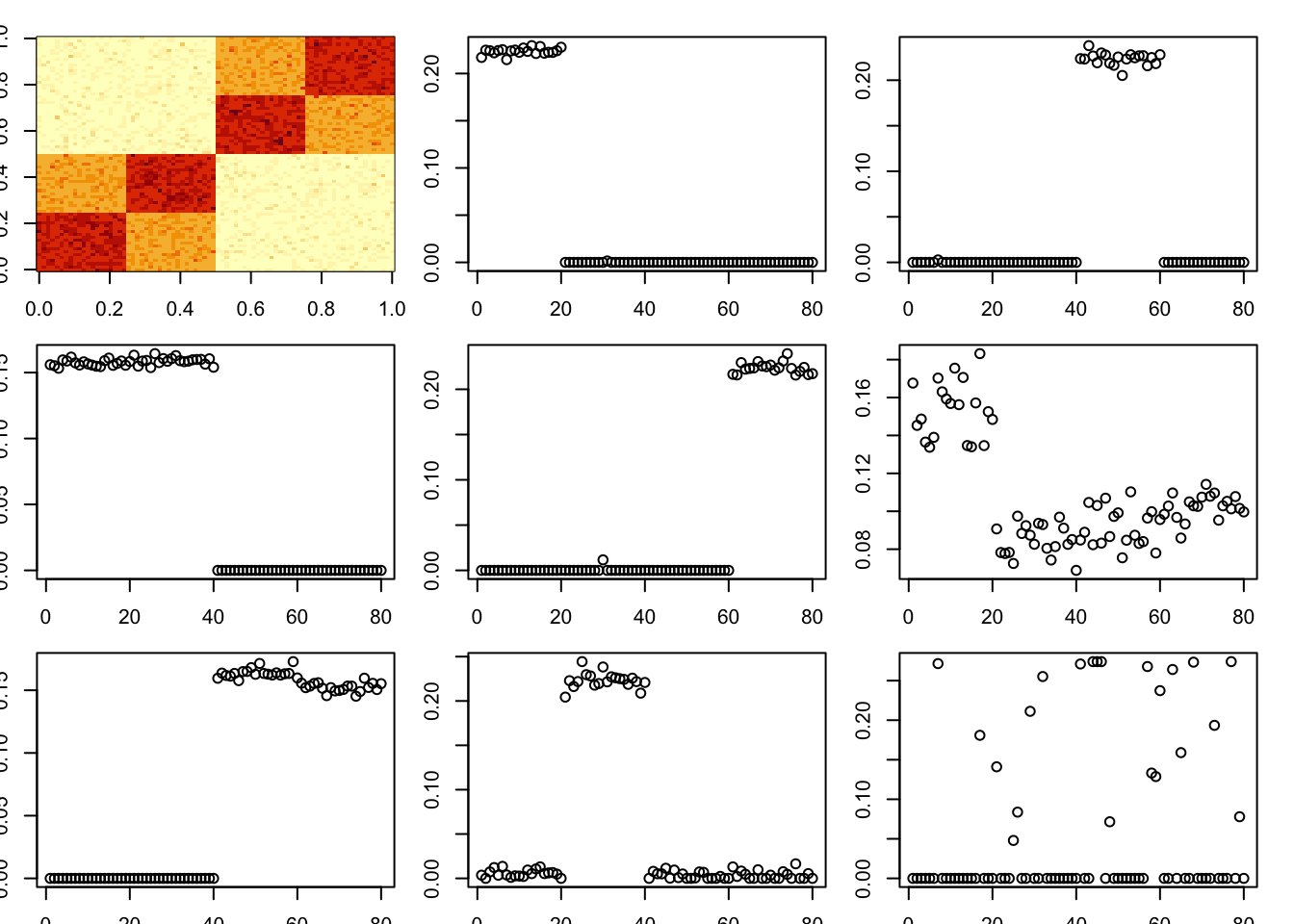
toc()

13.232 sec elapsed

Estimate sigma by mle (note that this is quite a bit slower).

A = x %*% t(x) + E
par(mfcol=c(3,3),mai=rep(0.2,4))
image(A)
tic()
for(i in 1:8){
  fit = nmu_em_estlambda(A,est.method = "mle.sigma")
  A = A-fit$d*fit$u %*% t(fit$u)
  fit$lambda
  fit$sigma
  plot(fit$u)
}

Past versions of unnamed-chunk-14-1.png

Version	Author	Date
8ac1380	Matthew Stephens	2025-02-27
eb0b82b	Matthew Stephens	2025-02-26

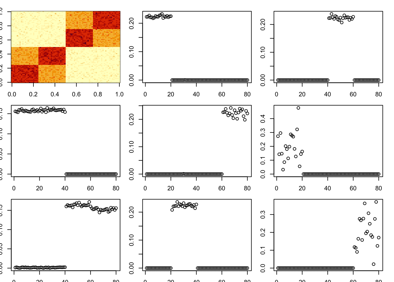
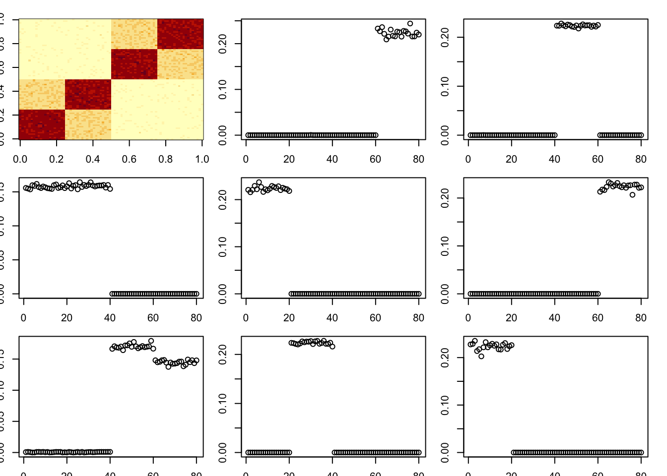
toc()

43.886 sec elapsed

Here I try a tree with a stronger diagonal; the idea is that this might cause it to remove the bottom branches first, which might break the whole thing? However it continues to work quite well.

set.seed(1)
n = 40
x = cbind(c(rep(1,n),rep(0,n)), c(rep(0,n),rep(1,n)), c(rep(1,n/2),rep(0,3*n/2)), c(rep(0,n/2), rep(1,n/2), rep(0,n)), c(rep(0,n),rep(1,n/2),rep(0,n/2)), c(rep(0,3*n/2),rep(1,n/2)))
E = matrix(0.1*rexp(2*n*2*n),nrow=2*n)
E = E+t(E) #symmetric errors

A = x %*% diag(c(1,1,3,3,3,3)) %*% t(x) + E
par(mfcol=c(3,3),mai=rep(0.2,4))
image(A)
tic()
for(i in 1:8){
  fit = nmu_em_estlambda(A,est.method = "mom")
  A = A-fit$d*fit$u %*% t(fit$u)
  fit$lambda
  fit$sigma
  plot(fit$u)
}

toc()

12.934 sec elapsed

A = x %*% diag(c(1,1,3,3,3,3)) %*% t(x) + E
par(mfcol=c(3,3),mai=rep(0.2,4))
image(A)
tic()
for(i in 1:8){
  fit = nmu_em_estlambda(A,est.method = "mle.sigma")
  A = A-fit$d*fit$u %*% t(fit$u)
  fit$lambda
  fit$sigma
  plot(fit$u)
}

toc()

47.595 sec elapsed

Here I try an even stronger diagonal. Interestingly it still does not totally break it (one factor becomes non-binar), and does not find the diagonal first.

A = x %*% diag(c(1,1,8,8,8,8)) %*% t(x) + E
par(mfcol=c(3,3),mai=rep(0.2,4))
image(A)
tic()
for(i in 1:8){
  fit = nmu_em_estlambda(A,est.method = "mom")
  A = A-fit$d*fit$u %*% t(fit$u)
  fit$lambda
  fit$sigma
  plot(fit$u)
}

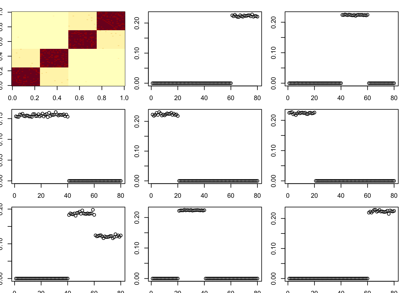
toc()

12.326 sec elapsed

Try mle.sigma

A = x %*% diag(c(1,1,8,8,8,8)) %*% t(x) + E
par(mfcol=c(3,3),mai=rep(0.2,4))
image(A)
tic()
for(i in 1:8){
  fit = nmu_em_estlambda(A,est.method = "mle.sigma")
  A = A-fit$d*fit$u %*% t(fit$u)
  fit$lambda
  fit$sigma
  plot(fit$u)
}

toc()

26.97 sec elapsed

Things to try

1. I think it could be possible to extend the prior on b to a mixture of exponentials (using code from ashr/ebnm for exponential mixtures). That might be worth trying.

2. One thought is that we could get a pretty good estimate of b from an initial low-rank approximation (eg PCA), and then do this process of NMU taking advantage of the known b. One motivation is to avoid the problem of overremoving things despite the nmu constraint - eg when it is a tree, but the bottom branches are found before the lower branches.

Here, as a first investigation of 2, I try initializing b using an SVD. This also allows me to easily fix lambda and sigma based on that estimated b. However, I found the results were very sensitive to the values of lambda and sigma, and also the number of iterations.

Here are the result for estimated lambda=0.37,sigma=0.12:

set.seed(1)
n = 40
x = cbind(c(rep(1,n),rep(0,n)), c(rep(0,n),rep(1,n)), c(rep(1,n/2),rep(0,3*n/2)), c(rep(0,n/2), rep(1,n/2), rep(0,n)), c(rep(0,n),rep(1,n/2),rep(0,n/2)), c(rep(0,3*n/2),rep(1,n/2)))
E = matrix(0.1*rexp(2*n*2*n),nrow=2*n)
E = E+t(E) #symmetric errors
A = x %*% diag(c(1,1,8,8,8,8)) %*% t(x) + E
A.svd = svd(A)
b = A.svd$u[,1:6] %*% diag(A.svd$d[1:6]) %*% t(A.svd$v[,1:6])

set.seed(2)
lambda = 1/mean(b)
sigma = sqrt(mean((A-b)^2))
lambda

[1] 0.3703403

sigma

[1] 0.1297278

u = rnorm(80)
for(i in 1:100){
  u = trunc_and_norm((A-b) %*% u)
  d = drop(t(u) %*% (A-b) %*% u)
  b = matrix(truncnorm::etruncnorm(a=0,mean= A-d*u %*% t(u)-lambda*sigma^2,sd=sigma),nrow=2*n)
}
plot(u)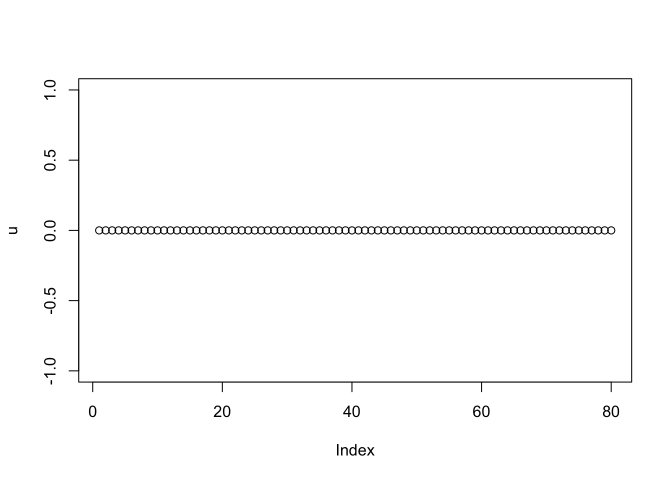

This is fixed lambda=1,sigma=0.1. Note that the results after 1000 iterations look pretty different from 100 iterations.

set.seed(2)
b = A.svd$u[,1:6] %*% diag(A.svd$d[1:6]) %*% t(A.svd$v[,1:6])
lambda = 1
sigma = 0.1
u = rnorm(80)
for(i in 1:100){
  u = trunc_and_norm((A-b) %*% u)
  d = drop(t(u) %*% (A-b) %*% u)
  b = matrix(truncnorm::etruncnorm(a=0,mean= A-d*u %*% t(u)-lambda*sigma^2,sd=sigma),nrow=2*n)
}
plot(u)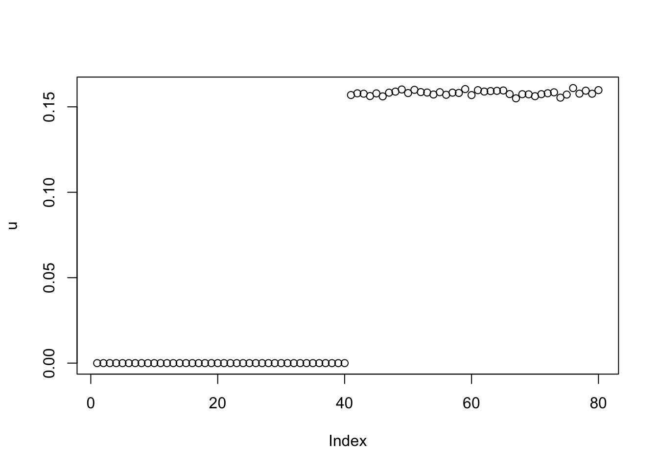

set.seed(2)
b = A.svd$u[,1:6] %*% diag(A.svd$d[1:6]) %*% t(A.svd$v[,1:6])
lambda = 1
sigma = 0.1
u = rnorm(80)
for(i in 1:1000){
  u = trunc_and_norm((A-b) %*% u)
  d = drop(t(u) %*% (A-b) %*% u)
  b = matrix(truncnorm::etruncnorm(a=0,mean= A-d*u %*% t(u)-lambda*sigma^2,sd=sigma),nrow=2*n)
}
plot(u)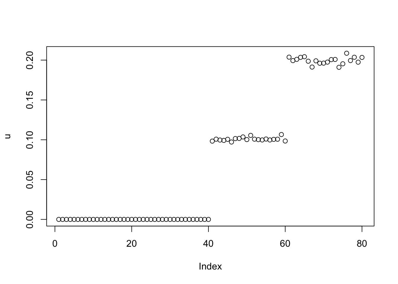

#lambda=1
#sigma=0.1

# par(mfcol=c(3,3))
# image(A)
# fit = nmu_em_estlambda(A,b.init=b)
# fit$lambda
# fit$sigma
# image(fit$u %*% t(fit$u))
# 
# A = A-fit$d*fit$u %*% t(fit$u)
# A.svd = svd(A)
# b = A.svd$u[,1:6] %*% diag(A.svd$d[1:6]) %*% t(A.svd$v[,1:6])
# 

# fit = nmu_em_estlambda(A,b.init=b)
# image(fit$u %*% t(fit$u))
# 
# A = A-fit$d*fit$u %*% t(fit$u)
# fit = nmu_em_estlambda(A)
# image(fit$u %*% t(fit$u))
# 
# A = A-fit$d*fit$u %*% t(fit$u)
# fit = nmu_em_estlambda(A)
# image(fit$u %*% t(fit$u))
# 
# A = A-fit$d*fit$u %*% t(fit$u)
# fit = nmu_em_estlambda(A)
# image(fit$u %*% t(fit$u))
# 
# A = A-fit$d*fit$u %*% t(fit$u)
# fit = nmu_em_estlambda(A)
# image(fit$u %*% t(fit$u))
# 
# A = A-fit$d*fit$u %*% t(fit$u)
# fit = nmu_em_estlambda(A)
# image(fit$u %*% t(fit$u))
# 
# A = A-fit$d*fit$u %*% t(fit$u)
# fit = nmu_em_estlambda(A)
# image(fit$u %*% t(fit$u))
# 

Further thoughts; scaling

I’m not entirely satisfied with the way we estimate lambda,sigma - that needs some thought I think.

Also, I note that the result can depend on the scale of \(A,\lambda, \sigma\). We might want to frame the problem a bit differently to avoid that… eg by \(A = \sigma(uv'+b+e)\) where \(e \sim N(0,1)\) and \(b \sim Exp(\lambda)\). This could help make the approach scale invariant – that is, multiplying A by a constant would effectively not change the solution – which seems desirable. (Another simpler way to do this would be to simply to scale A to have mean squared values of 1 before proceeding.)

We could try \[A = \sigma(uv' + b + e)\] where \(u,v\) non-negative, \(e \sim N(0,1)\) and \(b\sim Exp(lambda)\).

The ELBO is \[F(u,v,q)= E_q((-1/2\sigma^2)||A-\sigma uv'-\sigma b||_2^2) + D_{KL}(q,g)\] where \(g\) is the prior on \(b\), \[g(b)=\lambda \exp(-\lambda b).\] Here \(q\) plays the role of the (approximate) posterior distribution on \(b\).

Given \(q\), this is minimized for \(u,v\) by solving \[\min_{u,v} ||A/\sigma -\bar{b} - uv'||_2^2\]

Given \(u,v\) this is minimized by for each \(b_{ij}\) by solving \[q(b) \propto g(b) \exp((-1/2)(x_{ij} - b)^2) \propto \exp((-1/2)[b^2-2(x_{ij}-\lambda)b])\] where \(x_{ij} = A_ij/\sigma - u_i v_j\). This is a truncated normal distribution, \[q(b_{ij}) = N_+(x_{ij}-\lambda, 1)\].

Session information

sessionInfo()

R version 4.4.2 (2024-10-31)
Platform: aarch64-apple-darwin20
Running under: macOS Sequoia 15.3.1

Matrix products: default
BLAS:   /Library/Frameworks/R.framework/Versions/4.4-arm64/Resources/lib/libRblas.0.dylib 
LAPACK: /Library/Frameworks/R.framework/Versions/4.4-arm64/Resources/lib/libRlapack.dylib;  LAPACK version 3.12.0

locale:
[1] en_US.UTF-8/en_US.UTF-8/en_US.UTF-8/C/en_US.UTF-8/en_US.UTF-8

time zone: America/Chicago
tzcode source: internal

attached base packages:
[1] stats4    stats     graphics  grDevices utils     datasets  methods  
[8] base     

other attached packages:
[1] tictoc_1.2.1   emg_1.0.9      moments_0.14.1

loaded via a namespace (and not attached):
 [1] vctrs_0.6.5       cli_3.6.3         knitr_1.49        rlang_1.1.5      
 [5] xfun_0.50         stringi_1.8.4     promises_1.3.2    jsonlite_1.8.9   
 [9] workflowr_1.7.1   glue_1.8.0        rprojroot_2.0.4   git2r_0.35.0     
[13] htmltools_0.5.8.1 httpuv_1.6.15     sass_0.4.9        rmarkdown_2.29   
[17] evaluate_1.0.3    jquerylib_0.1.4   tibble_3.2.1      fastmap_1.2.0    
[21] yaml_2.3.10       lifecycle_1.0.4   whisker_0.4.1     stringr_1.5.1    
[25] compiler_4.4.2    fs_1.6.5          Rcpp_1.0.14       pkgconfig_2.0.3  
[29] rstudioapi_0.17.1 later_1.4.1       truncnorm_1.0-9   digest_0.6.37    
[33] R6_2.5.1          pillar_1.10.1     magrittr_2.0.3    bslib_0.9.0      
[37] tools_4.4.2       cachem_1.1.0