ridge_em_svd
Matthew Stephens
2020-06-26
Last updated: 2020-06-26
Checks: 7 0
Knit directory: misc/analysis/
This reproducible R Markdown analysis was created with workflowr (version 1.6.1). The Checks tab describes the reproducibility checks that were applied when the results were created. The Past versions tab lists the development history.
Great! Since the R Markdown file has been committed to the Git repository, you know the exact version of the code that produced these results.
Great job! The global environment was empty. Objects defined in the global environment can affect the analysis in your R Markdown file in unknown ways. For reproduciblity it’s best to always run the code in an empty environment.
The command set.seed(1) was run prior to running the code in the R Markdown file. Setting a seed ensures that any results that rely on randomness, e.g. subsampling or permutations, are reproducible.
Great job! Recording the operating system, R version, and package versions is critical for reproducibility.
Nice! There were no cached chunks for this analysis, so you can be confident that you successfully produced the results during this run.
Great job! Using relative paths to the files within your workflowr project makes it easier to run your code on other machines.
Great! You are using Git for version control. Tracking code development and connecting the code version to the results is critical for reproducibility.
The results in this page were generated with repository version d5544c4. See the Past versions tab to see a history of the changes made to the R Markdown and HTML files.
Note that you need to be careful to ensure that all relevant files for the analysis have been committed to Git prior to generating the results (you can use wflow_publish or wflow_git_commit). workflowr only checks the R Markdown file, but you know if there are other scripts or data files that it depends on. Below is the status of the Git repository when the results were generated:
Ignored files:
    Ignored:    .DS_Store
    Ignored:    .Rhistory
    Ignored:    .Rproj.user/
    Ignored:    analysis/.RData
    Ignored:    analysis/.Rhistory
    Ignored:    analysis/ALStruct_cache/
    Ignored:    data/.Rhistory
    Ignored:    data/pbmc/

Untracked files:
    Untracked:  .dropbox
    Untracked:  Icon
    Untracked:  analysis/GHstan.Rmd
    Untracked:  analysis/GTEX-cogaps.Rmd
    Untracked:  analysis/PACS.Rmd
    Untracked:  analysis/Rplot.png
    Untracked:  analysis/SPCAvRP.rmd
    Untracked:  analysis/admm_02.Rmd
    Untracked:  analysis/admm_03.Rmd
    Untracked:  analysis/compare-transformed-models.Rmd
    Untracked:  analysis/cormotif.Rmd
    Untracked:  analysis/cp_ash.Rmd
    Untracked:  analysis/eQTL.perm.rand.pdf
    Untracked:  analysis/eb_prepilot.Rmd
    Untracked:  analysis/eb_var.Rmd
    Untracked:  analysis/ebpmf1.Rmd
    Untracked:  analysis/flash_test_tree.Rmd
    Untracked:  analysis/ieQTL.perm.rand.pdf
    Untracked:  analysis/lasso_em_03.Rmd
    Untracked:  analysis/m6amash.Rmd
    Untracked:  analysis/mash_bhat_z.Rmd
    Untracked:  analysis/mash_ieqtl_permutations.Rmd
    Untracked:  analysis/mixsqp.Rmd
    Untracked:  analysis/mr.ash_lasso_init.Rmd
    Untracked:  analysis/mr.mash.test.Rmd
    Untracked:  analysis/mr_ash_modular.Rmd
    Untracked:  analysis/mr_ash_parameterization.Rmd
    Untracked:  analysis/mr_ash_pen.Rmd
    Untracked:  analysis/mr_ash_ridge.Rmd
    Untracked:  analysis/nejm.Rmd
    Untracked:  analysis/normalize.Rmd
    Untracked:  analysis/pbmc.Rmd
    Untracked:  analysis/poisson_transform.Rmd
    Untracked:  analysis/pseudodata.Rmd
    Untracked:  analysis/qrnotes.txt
    Untracked:  analysis/ridge_iterative_02.Rmd
    Untracked:  analysis/ridge_iterative_splitting.Rmd
    Untracked:  analysis/samps/
    Untracked:  analysis/sc_bimodal.Rmd
    Untracked:  analysis/shrinkage_comparisons_changepoints.Rmd
    Untracked:  analysis/susie_en.Rmd
    Untracked:  analysis/susie_z_investigate.Rmd
    Untracked:  analysis/svd-timing.Rmd
    Untracked:  analysis/temp.RDS
    Untracked:  analysis/temp.Rmd
    Untracked:  analysis/test-figure/
    Untracked:  analysis/test.Rmd
    Untracked:  analysis/test.Rpres
    Untracked:  analysis/test.md
    Untracked:  analysis/test_qr.R
    Untracked:  analysis/test_sparse.Rmd
    Untracked:  analysis/z.txt
    Untracked:  code/multivariate_testfuncs.R
    Untracked:  code/rqb.hacked.R
    Untracked:  data/4matthew/
    Untracked:  data/4matthew2/
    Untracked:  data/E-MTAB-2805.processed.1/
    Untracked:  data/ENSG00000156738.Sim_Y2.RDS
    Untracked:  data/GDS5363_full.soft.gz
    Untracked:  data/GSE41265_allGenesTPM.txt
    Untracked:  data/Muscle_Skeletal.ACTN3.pm1Mb.RDS
    Untracked:  data/Thyroid.FMO2.pm1Mb.RDS
    Untracked:  data/bmass.HaemgenRBC2016.MAF01.Vs2.MergedDataSources.200kRanSubset.ChrBPMAFMarkerZScores.vs1.txt.gz
    Untracked:  data/bmass.HaemgenRBC2016.Vs2.NewSNPs.ZScores.hclust.vs1.txt
    Untracked:  data/bmass.HaemgenRBC2016.Vs2.PreviousSNPs.ZScores.hclust.vs1.txt
    Untracked:  data/eb_prepilot/
    Untracked:  data/finemap_data/fmo2.sim/b.txt
    Untracked:  data/finemap_data/fmo2.sim/dap_out.txt
    Untracked:  data/finemap_data/fmo2.sim/dap_out2.txt
    Untracked:  data/finemap_data/fmo2.sim/dap_out2_snp.txt
    Untracked:  data/finemap_data/fmo2.sim/dap_out_snp.txt
    Untracked:  data/finemap_data/fmo2.sim/data
    Untracked:  data/finemap_data/fmo2.sim/fmo2.sim.config
    Untracked:  data/finemap_data/fmo2.sim/fmo2.sim.k
    Untracked:  data/finemap_data/fmo2.sim/fmo2.sim.k4.config
    Untracked:  data/finemap_data/fmo2.sim/fmo2.sim.k4.snp
    Untracked:  data/finemap_data/fmo2.sim/fmo2.sim.ld
    Untracked:  data/finemap_data/fmo2.sim/fmo2.sim.snp
    Untracked:  data/finemap_data/fmo2.sim/fmo2.sim.z
    Untracked:  data/finemap_data/fmo2.sim/pos.txt
    Untracked:  data/logm.csv
    Untracked:  data/m.cd.RDS
    Untracked:  data/m.cdu.old.RDS
    Untracked:  data/m.new.cd.RDS
    Untracked:  data/m.old.cd.RDS
    Untracked:  data/mainbib.bib.old
    Untracked:  data/mat.csv
    Untracked:  data/mat.txt
    Untracked:  data/mat_new.csv
    Untracked:  data/matrix_lik.rds
    Untracked:  data/paintor_data/
    Untracked:  data/temp.txt
    Untracked:  data/y.txt
    Untracked:  data/y_f.txt
    Untracked:  data/zscore_jointLCLs_m6AQTLs_susie_eQTLpruned.rds
    Untracked:  data/zscore_jointLCLs_random.rds
    Untracked:  explore_udi.R
    Untracked:  output/fit.k10.rds
    Untracked:  output/fit.varbvs.RDS
    Untracked:  output/glmnet.fit.RDS
    Untracked:  output/test.bv.txt
    Untracked:  output/test.gamma.txt
    Untracked:  output/test.hyp.txt
    Untracked:  output/test.log.txt
    Untracked:  output/test.param.txt
    Untracked:  output/test2.bv.txt
    Untracked:  output/test2.gamma.txt
    Untracked:  output/test2.hyp.txt
    Untracked:  output/test2.log.txt
    Untracked:  output/test2.param.txt
    Untracked:  output/test3.bv.txt
    Untracked:  output/test3.gamma.txt
    Untracked:  output/test3.hyp.txt
    Untracked:  output/test3.log.txt
    Untracked:  output/test3.param.txt
    Untracked:  output/test4.bv.txt
    Untracked:  output/test4.gamma.txt
    Untracked:  output/test4.hyp.txt
    Untracked:  output/test4.log.txt
    Untracked:  output/test4.param.txt
    Untracked:  output/test5.bv.txt
    Untracked:  output/test5.gamma.txt
    Untracked:  output/test5.hyp.txt
    Untracked:  output/test5.log.txt
    Untracked:  output/test5.param.txt

Unstaged changes:
    Modified:   analysis/ash_delta_operator.Rmd
    Modified:   analysis/ash_pois_bcell.Rmd
    Modified:   analysis/lasso_em.Rmd
    Modified:   analysis/minque.Rmd
    Modified:   analysis/mr_missing_data.Rmd
Note that any generated files, e.g. HTML, png, CSS, etc., are not included in this status report because it is ok for generated content to have uncommitted changes.
These are the previous versions of the repository in which changes were made to the R Markdown (analysis/ridge_em_svd.Rmd) and HTML (docs/ridge_em_svd.html) files. If you’ve configured a remote Git repository (see ?wflow_git_remote), click on the hyperlinks in the table below to view the files as they were in that past version.
| File | Version | Author | Date | Message |
|---|---|---|---|---|
| Rmd | d5544c4 | Matthew Stephens | 2020-06-26 | workflowr::wflow_publish(“ridge_em_svd.Rmd”) |
| html | 7e50690 | Matthew Stephens | 2020-06-26 | Build site. |
| Rmd | fab7fde | Matthew Stephens | 2020-06-26 | workflowr::wflow_publish(“ridge_em_svd.Rmd”) |
| html | ae73528 | Matthew Stephens | 2020-06-26 | Build site. |
| Rmd | ced143f | Matthew Stephens | 2020-06-26 | workflowr::wflow_publish(“ridge_em_svd.Rmd”) |
| html | 29360cf | Matthew Stephens | 2020-06-26 | Build site. |
| Rmd | 25cb420 | Matthew Stephens | 2020-06-26 | workflowr::wflow_publish(“ridge_em_svd.Rmd”) |
Introduction
Following up on these EM algorithms to fit Ridge by EB, I look at implementing these kinds of ideas when an SVD for \(X=UDV'\) is available (or, simply by doing SVD of \(X\) as a pre-computation step). Note that randomized methods can allow very fast approximation of the SVD of \(X\) for large matrices, and I have in mind we may be able to exploit these down the line, especially as we may only need approximate solutions to ridge regression for our purposes.
I assume we are in the big \(p\) regime, so \(D\) is \(k\) \(k\) with \(k<p\), and \(V'V = I_k\), and \(U'U=I_k\). Often we will have \(k=n\), in which case \(UU'= U'U = I_n\).
The model is: \[Y \sim N(Xb, s^2I_n)\]
Premultiplying by \(U'\) gives: \[U'Y \sim N(DV'b, s^2 I_k)\] which we can write as \[\tilde{Y}_j \sim N(\theta_j, s^2)\] \[\theta_j \sim N(0, s_b^2 d_j^2)\].
And we can solve this by EM, just as before. Of course we can parameterize in various ways.
Some derivations are here.
Here is the EM for the simple parameterization as above:
ridge_indep_em1 = function(y, d2, s2, sb2, niter=10){
  k = length(y)
  loglik = rep(0,niter)

  for(i in 1:niter){

    prior_var = sb2*d2
    data_var = s2

    loglik[i] = sum(dnorm(y,mean=0,sd = sqrt(sb2*d2 + s2),log=TRUE))

    # update sb2
    post_var = 1/((1/prior_var) + (1/data_var)) #posterior variance of theta
    post_mean =  post_var * (1/data_var) * y # posterior mean of theta
    sb2 = mean((post_mean^2 + post_var)/d2)

    # update s2
    r = y - post_mean # residuals
    s2 = mean(r^2 + post_var)
  }
  return(list(s2=s2,sb2=sb2,loglik=loglik,postmean = post_mean))
}
Scaled parameterization
Here we take the \(s_b\) out of the prior on \(\theta_j\): \[y_j \sim N(s_b \theta_j, s^2)\] \[\theta_j \sim N(0,d_j^2).\]
Note that we could also put the \(d_j\) into the mean of \(y_j\) and have \(\theta_j \sim N(0,1)\) but this ends up leading to exactly the same EM algorithm. (In earlier versions of this document I implemented this, but it turned out to indeed be identical, so I removed it.)
Note also that here I give the option to recompute quantities between updates of sb2 and s2. However, this didn’t help in any examples I tried (not shown).
ridge_indep_em2 = function(y, d2, s2, sb2, niter=10, recompute_between_updates = FALSE){
  k = length(y)
  loglik = rep(0,niter)
  for(i in 1:niter){
    loglik[i] = sum(dnorm(y,mean=0,sd = sqrt(sb2*d2 + s2),log=TRUE))

    prior_var = d2 # prior variance for theta
    data_var = s2/sb2 # variance of y/sb, which has mean theta
    post_var = 1/((1/prior_var) + (1/data_var)) #posterior variance of theta
    post_mean =  post_var * (1/data_var) * (y/sqrt(sb2)) # posterior mean of theta

    sb2 = (sum(y*post_mean)/sum(post_mean^2 + post_var))^2

    if(recompute_between_updates){
      prior_var = d2 # prior variance for theta
      data_var = s2/sb2 # variance of y/sb, which has mean theta
      post_var = 1/((1/prior_var) + (1/data_var)) #posterior variance of theta
      post_mean =  post_var * (1/data_var) * (y/sqrt(sb2)) # posterior mean of theta
    }

    r = y - sqrt(sb2) * post_mean # residuals
    s2 = mean(r^2 + sb2 * post_var)

  }
  return(list(s2=s2,sb2=sb2,loglik=loglik,postmean = sqrt(sb2) * post_mean))
}
Hybrid/redundant parameterization
As before we take a hybrid approach aimed at getting the best of both worlds.
\[y_j \sim N(s_b \theta_j, s^2)\] \[\theta_j \sim N(0,l^2 d_j^2).\] The updates involve combinations of the updates in em1 and em2.
ridge_indep_em3 = function(y, d2, s2, sb2, l2,niter=10){
  k = length(y)
  loglik = rep(0,niter)
  for(i in 1:niter){
    loglik[i] = sum(dnorm(y,mean=0,sd = sqrt(sb2*l2*d2 + s2),log=TRUE))

    prior_var = d2*l2 # prior variance for theta
    data_var = s2/sb2 # variance of y/sb, which has mean theta
    post_var = 1/((1/prior_var) + (1/data_var)) #posterior variance of theta
    post_mean =  post_var * (1/data_var) * (y/sqrt(sb2)) # posterior mean of theta

    sb2 = (sum(y*post_mean)/sum(post_mean^2 + post_var))^2
    l2 = mean((post_mean^2 + post_var)/d2)

    r = y - sqrt(sb2) * post_mean # residuals
    s2 = mean(r^2 + sb2 * post_var)

  }
  return(list(s2=s2,sb2=sb2,loglik=loglik,postmean = sqrt(sb2) *post_mean))
}
Simple simulation
Here we try a simple simulation to test:
set.seed(100)
sd = 1
n = 100
p = n
X = matrix(rnorm(n*p),ncol=n)
btrue = rnorm(n)
y = X %*% btrue + sd*rnorm(n)

plot(X %*% btrue, y)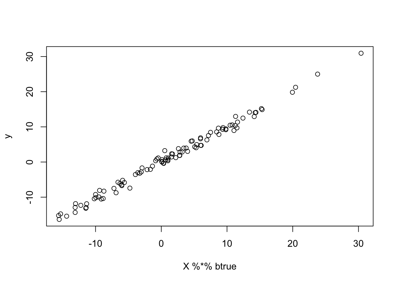
Here I define a function to plot the log-likelihoods:
plot_loglik = function(res){
  maxloglik = max(res[[1]]$loglik)
  minloglik = min(res[[1]]$loglik)
  maxlen =length(res[[1]]$loglik)
  for(i in 2:length(res)){
    maxloglik = max(c(maxloglik,res[[i]]$loglik))
    minloglik = min(c(minloglik,res[[i]]$loglik))
    maxlen= max(maxlen, length(res[[i]]$loglik))
  }


  plot(res[[1]]$loglik,type="n",ylim=c(minloglik,maxloglik),xlim=c(0,maxlen),ylab="log-likelihood",
       xlab="iteration")
  for(i in 1:length(res)){
    lines(res[[i]]$loglik,col=i,lwd=2)
  }

}
Run all the methods: the scaled parameterization is worst here:
X.svd = svd(X)
ytilde = drop(t(X.svd$u) %*% y)
yt.em1 = ridge_indep_em1(ytilde,X.svd$d^2,1,1,100)
yt.em2 = ridge_indep_em2(ytilde,X.svd$d^2,1,1,100)
yt.em3= ridge_indep_em3(ytilde,X.svd$d^2,1,1,1,100)

plot_loglik(list(yt.em1,yt.em2,yt.em3))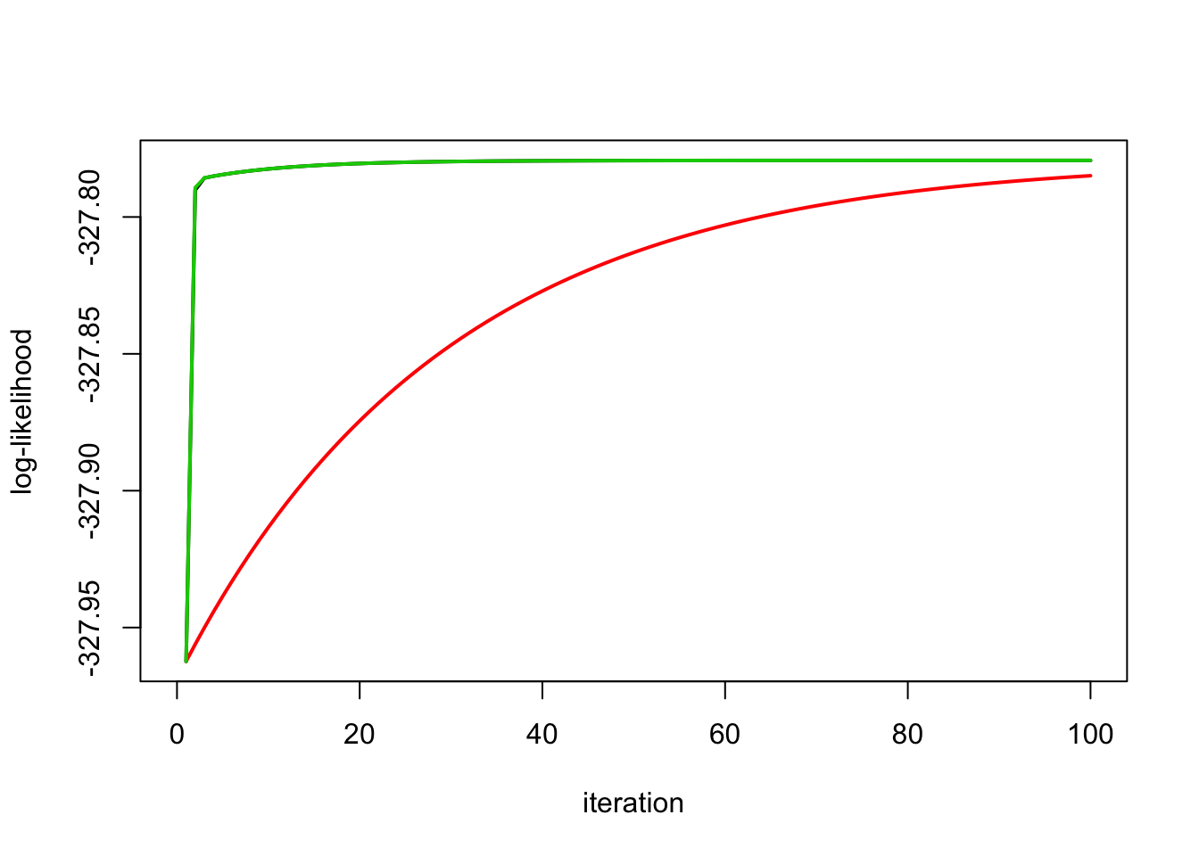
Check that the posterior means are all the same
plot(ytilde, yt.em1$postmean,col=1)
points(ytilde, yt.em2$postmean,col=2)
points(ytilde, yt.em3$postmean,col=3)
abline(a=0,b=1)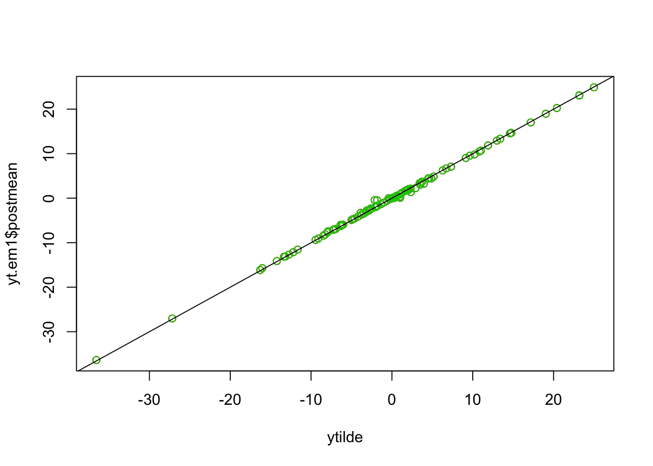
Try different initializations. Here s2=.1 and sb2=10.
yt.em1 = ridge_indep_em1(ytilde,X.svd$d^2,.1,10,100)
yt.em2 = ridge_indep_em2(ytilde,X.svd$d^2,.1,10,100)
yt.em3= ridge_indep_em3(ytilde,X.svd$d^2,.1,10,1,100)

plot_loglik(list(yt.em1,yt.em2,yt.em3))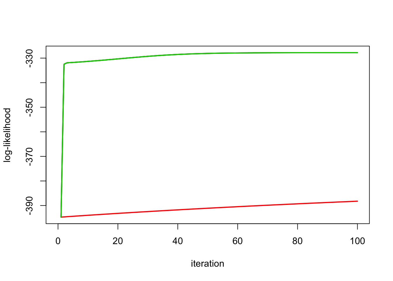
Here s2=10 and sb2=.1.
yt.em1 = ridge_indep_em1(ytilde,X.svd$d^2,10,.1,50)
yt.em2 = ridge_indep_em2(ytilde,X.svd$d^2,10,.1,50)
yt.em3= ridge_indep_em3(ytilde,X.svd$d^2,10,.1,1,50)

plot_loglik(list(yt.em1,yt.em2,yt.em3))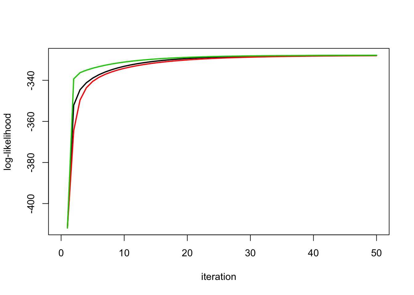
No signal
This simulation has no signal (b=0). Methods are similar here.
btrue = rep(0,n)
y = X %*% btrue + sd*rnorm(n)

X.svd = svd(X)
ytilde = drop(t(X.svd$u) %*% y)
yt.em1 = ridge_indep_em1(ytilde,X.svd$d^2,1,1,100)
yt.em2 = ridge_indep_em2(ytilde,X.svd$d^2,1,1,100)
yt.em3 = ridge_indep_em3(ytilde,X.svd$d^2,1,1,1,100)


plot_loglik(list(yt.em1,yt.em2,yt.em3))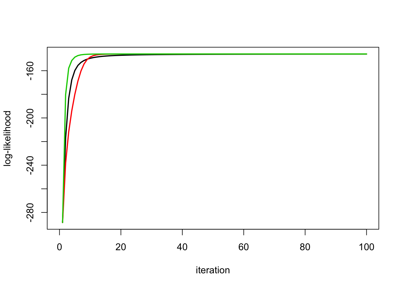
Trendfiltering Simulations
This is more challenging example (in that the design matrix is correlated)
High Signal
set.seed(100)
sd = 1
n = 100
p = n
X = matrix(0,nrow=n,ncol=n)
for(i in 1:n){
  X[i:n,i] = 1:(n-i+1)
}
btrue = rep(0,n)
btrue[40] = 8
btrue[41] = -8
y = X %*% btrue + sd*rnorm(n)

plot(y)
lines(X %*% btrue)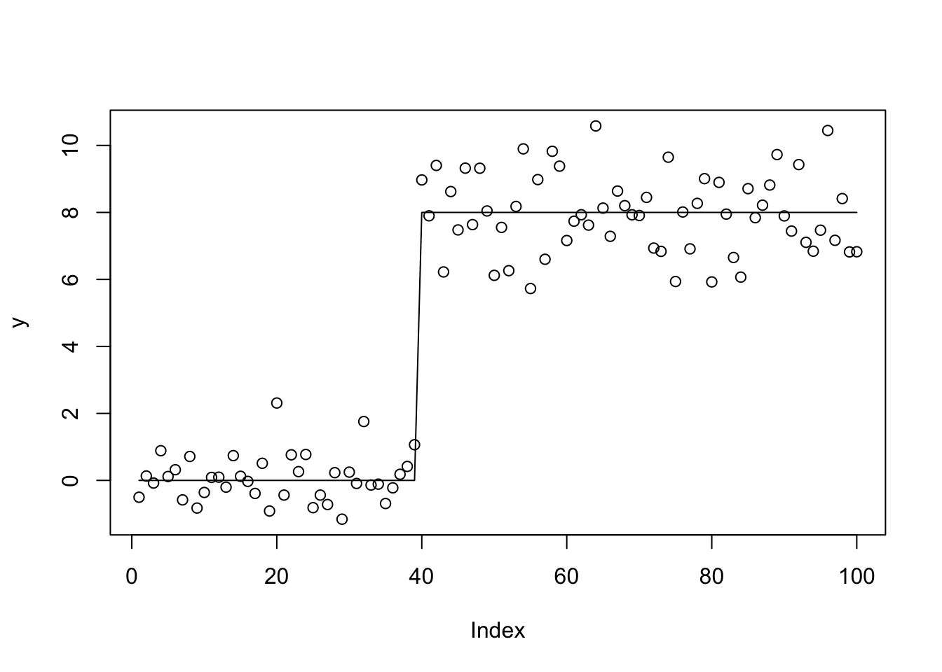
| Version | Author | Date |
|---|---|---|
| 7e50690 | Matthew Stephens | 2020-06-26 |
Run the methods: there is a clear advantage of simple parameterization.
X.svd = svd(X)
ytilde = drop(t(X.svd$u) %*% y)

yt.em1 = ridge_indep_em1(ytilde,X.svd$d^2,1,1,100)
yt.em2 = ridge_indep_em2(ytilde,X.svd$d^2,1,1,100)
yt.em3 = ridge_indep_em3(ytilde,X.svd$d^2,1,1,1,100)

plot_loglik(list(yt.em1,yt.em2,yt.em3))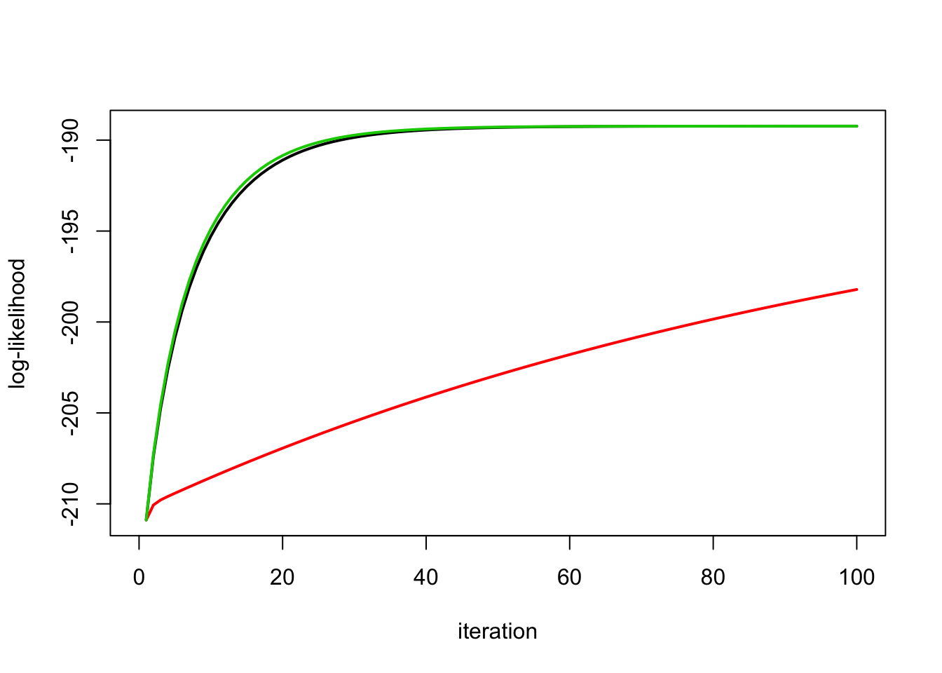
| Version | Author | Date |
|---|---|---|
| 7e50690 | Matthew Stephens | 2020-06-26 |
Fits are different:
plot(y)
lines(X %*% btrue,col="gray")
lines(X.svd$u %*% yt.em1$postmean,lwd=2)
lines(X.svd$u %*% yt.em2$postmean,col=2,lwd=2)
lines(X.svd$u %*% yt.em3$postmean,col=3,lwd=2)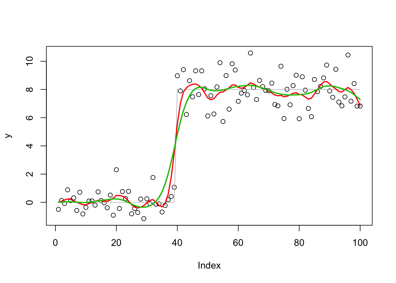
No signal case
Try no signal case
sd = 1
n = 100
p = n
X = matrix(0,nrow=n,ncol=n)
for(i in 1:n){
  X[i:n,i] = 1:(n-i+1)
}
btrue = rep(0,n)

y = X %*% btrue + sd*rnorm(n)

plot(y)
lines(X %*% btrue)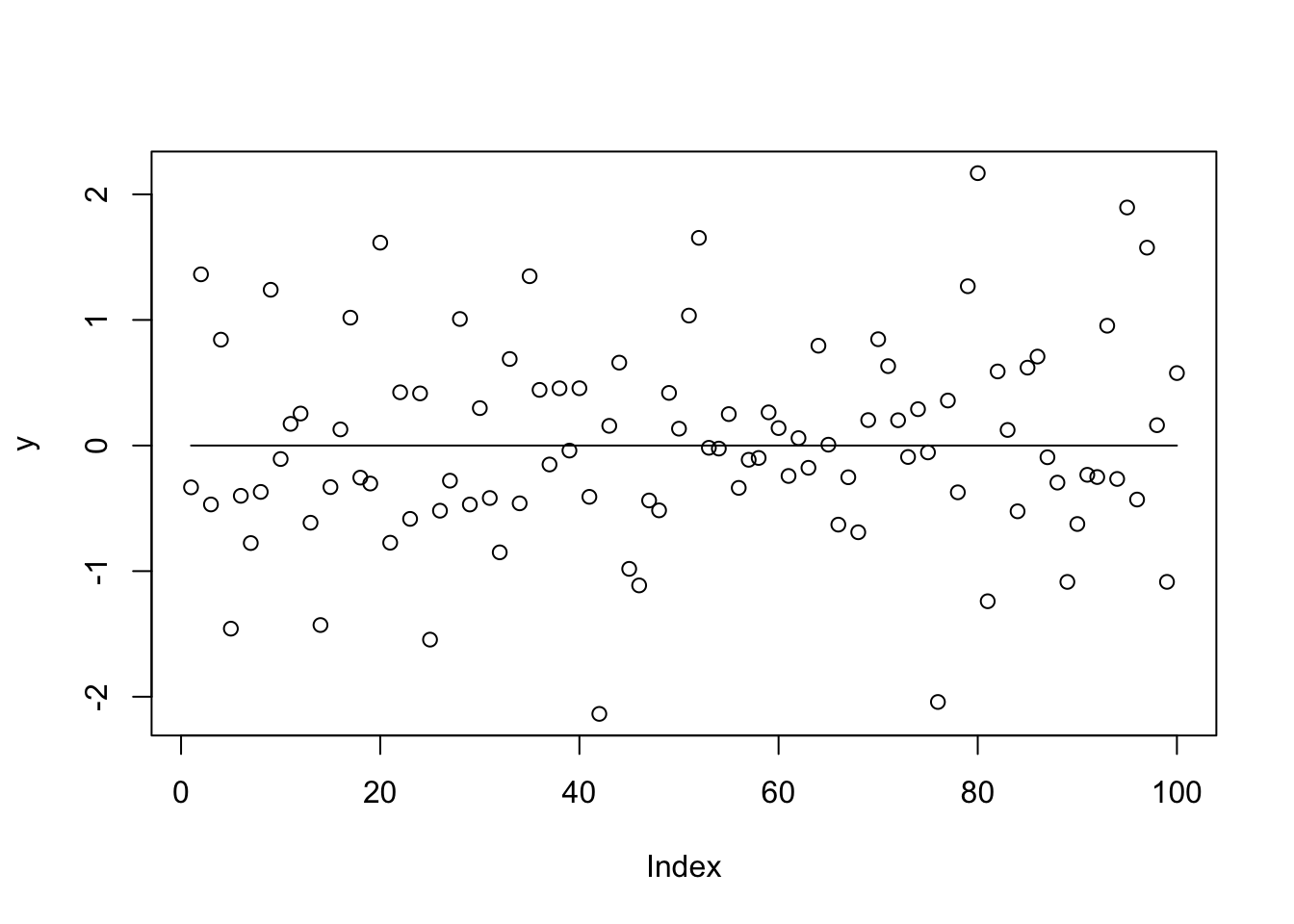
Run the EM: there is a clear advantage of scaled parameterizations.
X.svd = svd(X)
ytilde = drop(t(X.svd$u) %*% y)

yt.em1 = ridge_indep_em1(ytilde,X.svd$d^2,1,1,100)
yt.em2 = ridge_indep_em2(ytilde,X.svd$d^2,1,1,100)
yt.em3 = ridge_indep_em3(ytilde,X.svd$d^2,1,1,1,100)

plot_loglik(list(yt.em1,yt.em2,yt.em3))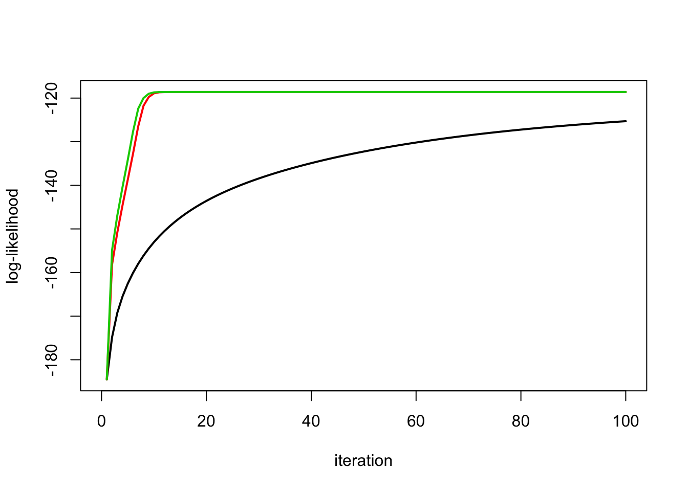
sessionInfo()R version 3.6.0 (2019-04-26)
Platform: x86_64-apple-darwin15.6.0 (64-bit)
Running under: macOS Mojave 10.14.6
Matrix products: default
BLAS: /Library/Frameworks/R.framework/Versions/3.6/Resources/lib/libRblas.0.dylib
LAPACK: /Library/Frameworks/R.framework/Versions/3.6/Resources/lib/libRlapack.dylib
locale:
[1] en_US.UTF-8/en_US.UTF-8/en_US.UTF-8/C/en_US.UTF-8/en_US.UTF-8
attached base packages:
[1] stats graphics grDevices utils datasets methods base
loaded via a namespace (and not attached):
[1] workflowr_1.6.1 Rcpp_1.0.4.6 rprojroot_1.3-2 digest_0.6.25
[5] later_1.0.0 R6_2.4.1 backports_1.1.5 git2r_0.26.1
[9] magrittr_1.5 evaluate_0.14 stringi_1.4.6 rlang_0.4.5
[13] fs_1.3.2 promises_1.1.0 whisker_0.4 rmarkdown_2.1
[17] tools_3.6.0 stringr_1.4.0 glue_1.4.0 httpuv_1.5.2
[21] xfun_0.12 yaml_2.2.1 compiler_3.6.0 htmltools_0.4.0
[25] knitr_1.28