tree_ebcd

workflowr

• Summary
• Checks
• Past versions

Last updated: 2024-09-14

Checks: 7 0

Knit directory: misc/analysis/

This reproducible R Markdown analysis was created with workflowr (version 1.7.1). The Checks tab describes the reproducibility checks that were applied when the results were created. The Past versions tab lists the development history.

---

R Markdown file: up-to-date

Great! Since the R Markdown file has been committed to the Git repository, you know the exact version of the code that produced these results.

Environment: empty

Great job! The global environment was empty. Objects defined in the global environment can affect the analysis in your R Markdown file in unknown ways. For reproduciblity it’s best to always run the code in an empty environment.

Seed: set.seed(1)

The command set.seed(1) was run prior to running the code in the R Markdown file. Setting a seed ensures that any results that rely on randomness, e.g. subsampling or permutations, are reproducible.

Session information: recorded

Great job! Recording the operating system, R version, and package versions is critical for reproducibility.

Cache: none

Nice! There were no cached chunks for this analysis, so you can be confident that you successfully produced the results during this run.

File paths: relative

Great job! Using relative paths to the files within your workflowr project makes it easier to run your code on other machines.

Repository version: 596ea6a

Great! You are using Git for version control. Tracking code development and connecting the code version to the results is critical for reproducibility.

The results in this page were generated with repository version 596ea6a. See the Past versions tab to see a history of the changes made to the R Markdown and HTML files.

Note that you need to be careful to ensure that all relevant files for the analysis have been committed to Git prior to generating the results (you can use wflow_publish or wflow_git_commit). workflowr only checks the R Markdown file, but you know if there are other scripts or data files that it depends on. Below is the status of the Git repository when the results were generated:

Ignored files:
    Ignored:    .DS_Store
    Ignored:    .Rhistory
    Ignored:    .Rproj.user/
    Ignored:    analysis/.RData
    Ignored:    analysis/.Rhistory
    Ignored:    analysis/ALStruct_cache/
    Ignored:    data/.Rhistory
    Ignored:    data/methylation-data-for-matthew.rds
    Ignored:    data/pbmc/
    Ignored:    data/pbmc_purified.RData

Untracked files:
    Untracked:  .dropbox
    Untracked:  Icon
    Untracked:  analysis/GHstan.Rmd
    Untracked:  analysis/GTEX-cogaps.Rmd
    Untracked:  analysis/PACS.Rmd
    Untracked:  analysis/Rplot.png
    Untracked:  analysis/SPCAvRP.rmd
    Untracked:  analysis/abf_comparisons.Rmd
    Untracked:  analysis/admm_02.Rmd
    Untracked:  analysis/admm_03.Rmd
    Untracked:  analysis/cache/
    Untracked:  analysis/cholesky.Rmd
    Untracked:  analysis/compare-transformed-models.Rmd
    Untracked:  analysis/cormotif.Rmd
    Untracked:  analysis/cp_ash.Rmd
    Untracked:  analysis/eQTL.perm.rand.pdf
    Untracked:  analysis/eb_prepilot.Rmd
    Untracked:  analysis/eb_var.Rmd
    Untracked:  analysis/ebpmf1.Rmd
    Untracked:  analysis/ebpmf_sla_text.Rmd
    Untracked:  analysis/ebspca_sims.Rmd
    Untracked:  analysis/explore_psvd.Rmd
    Untracked:  analysis/fa_check_identify.Rmd
    Untracked:  analysis/fa_iterative.Rmd
    Untracked:  analysis/flash_test_tree.Rmd
    Untracked:  analysis/flash_tree.Rmd
    Untracked:  analysis/flashier_newgroups.Rmd
    Untracked:  analysis/flashier_nmf_triples.Rmd
    Untracked:  analysis/flashier_pbmc.Rmd
    Untracked:  analysis/flashier_snn_shifted_prior.Rmd
    Untracked:  analysis/greedy_ebpmf_exploration_00.Rmd
    Untracked:  analysis/ieQTL.perm.rand.pdf
    Untracked:  analysis/lasso_em_03.Rmd
    Untracked:  analysis/m6amash.Rmd
    Untracked:  analysis/mash_bhat_z.Rmd
    Untracked:  analysis/mash_ieqtl_permutations.Rmd
    Untracked:  analysis/methylation_example.Rmd
    Untracked:  analysis/mixsqp.Rmd
    Untracked:  analysis/mr.ash_lasso_init.Rmd
    Untracked:  analysis/mr.mash.test.Rmd
    Untracked:  analysis/mr_ash_modular.Rmd
    Untracked:  analysis/mr_ash_parameterization.Rmd
    Untracked:  analysis/mr_ash_ridge.Rmd
    Untracked:  analysis/mv_gaussian_message_passing.Rmd
    Untracked:  analysis/nejm.Rmd
    Untracked:  analysis/nmf_bg.Rmd
    Untracked:  analysis/normal_conditional_on_r2.Rmd
    Untracked:  analysis/normalize.Rmd
    Untracked:  analysis/pbmc.Rmd
    Untracked:  analysis/pca_binary_weighted.Rmd
    Untracked:  analysis/pca_l1.Rmd
    Untracked:  analysis/poisson_nmf_approx.Rmd
    Untracked:  analysis/poisson_shrink.Rmd
    Untracked:  analysis/poisson_transform.Rmd
    Untracked:  analysis/qrnotes.txt
    Untracked:  analysis/ridge_iterative_02.Rmd
    Untracked:  analysis/ridge_iterative_splitting.Rmd
    Untracked:  analysis/samps/
    Untracked:  analysis/sc_bimodal.Rmd
    Untracked:  analysis/shrinkage_comparisons_changepoints.Rmd
    Untracked:  analysis/susie_cov.Rmd
    Untracked:  analysis/susie_en.Rmd
    Untracked:  analysis/susie_z_investigate.Rmd
    Untracked:  analysis/svd-timing.Rmd
    Untracked:  analysis/temp.RDS
    Untracked:  analysis/temp.Rmd
    Untracked:  analysis/test-figure/
    Untracked:  analysis/test.Rmd
    Untracked:  analysis/test.Rpres
    Untracked:  analysis/test.md
    Untracked:  analysis/test_qr.R
    Untracked:  analysis/test_sparse.Rmd
    Untracked:  analysis/tree_dist_top_eigenvector.Rmd
    Untracked:  analysis/z.txt
    Untracked:  code/multivariate_testfuncs.R
    Untracked:  code/rqb.hacked.R
    Untracked:  data/4matthew/
    Untracked:  data/4matthew2/
    Untracked:  data/E-MTAB-2805.processed.1/
    Untracked:  data/ENSG00000156738.Sim_Y2.RDS
    Untracked:  data/GDS5363_full.soft.gz
    Untracked:  data/GSE41265_allGenesTPM.txt
    Untracked:  data/Muscle_Skeletal.ACTN3.pm1Mb.RDS
    Untracked:  data/P.rds
    Untracked:  data/Thyroid.FMO2.pm1Mb.RDS
    Untracked:  data/bmass.HaemgenRBC2016.MAF01.Vs2.MergedDataSources.200kRanSubset.ChrBPMAFMarkerZScores.vs1.txt.gz
    Untracked:  data/bmass.HaemgenRBC2016.Vs2.NewSNPs.ZScores.hclust.vs1.txt
    Untracked:  data/bmass.HaemgenRBC2016.Vs2.PreviousSNPs.ZScores.hclust.vs1.txt
    Untracked:  data/eb_prepilot/
    Untracked:  data/finemap_data/fmo2.sim/b.txt
    Untracked:  data/finemap_data/fmo2.sim/dap_out.txt
    Untracked:  data/finemap_data/fmo2.sim/dap_out2.txt
    Untracked:  data/finemap_data/fmo2.sim/dap_out2_snp.txt
    Untracked:  data/finemap_data/fmo2.sim/dap_out_snp.txt
    Untracked:  data/finemap_data/fmo2.sim/data
    Untracked:  data/finemap_data/fmo2.sim/fmo2.sim.config
    Untracked:  data/finemap_data/fmo2.sim/fmo2.sim.k
    Untracked:  data/finemap_data/fmo2.sim/fmo2.sim.k4.config
    Untracked:  data/finemap_data/fmo2.sim/fmo2.sim.k4.snp
    Untracked:  data/finemap_data/fmo2.sim/fmo2.sim.ld
    Untracked:  data/finemap_data/fmo2.sim/fmo2.sim.snp
    Untracked:  data/finemap_data/fmo2.sim/fmo2.sim.z
    Untracked:  data/finemap_data/fmo2.sim/pos.txt
    Untracked:  data/logm.csv
    Untracked:  data/m.cd.RDS
    Untracked:  data/m.cdu.old.RDS
    Untracked:  data/m.new.cd.RDS
    Untracked:  data/m.old.cd.RDS
    Untracked:  data/mainbib.bib.old
    Untracked:  data/mat.csv
    Untracked:  data/mat.txt
    Untracked:  data/mat_new.csv
    Untracked:  data/matrix_lik.rds
    Untracked:  data/paintor_data/
    Untracked:  data/running_data_chris.csv
    Untracked:  data/running_data_matthew.csv
    Untracked:  data/temp.txt
    Untracked:  data/y.txt
    Untracked:  data/y_f.txt
    Untracked:  data/zscore_jointLCLs_m6AQTLs_susie_eQTLpruned.rds
    Untracked:  data/zscore_jointLCLs_random.rds
    Untracked:  explore_udi.R
    Untracked:  output/fit.k10.rds
    Untracked:  output/fit.nn.pbmc.purified.rds
    Untracked:  output/fit.nn.rds
    Untracked:  output/fit.nn.s.001.rds
    Untracked:  output/fit.nn.s.01.rds
    Untracked:  output/fit.nn.s.1.rds
    Untracked:  output/fit.nn.s.10.rds
    Untracked:  output/fit.snn.s.001.rds
    Untracked:  output/fit.snn.s.01.nninit.rds
    Untracked:  output/fit.snn.s.01.rds
    Untracked:  output/fit.varbvs.RDS
    Untracked:  output/fit2.nn.pbmc.purified.rds
    Untracked:  output/glmnet.fit.RDS
    Untracked:  output/snn07.txt
    Untracked:  output/snn34.txt
    Untracked:  output/test.bv.txt
    Untracked:  output/test.gamma.txt
    Untracked:  output/test.hyp.txt
    Untracked:  output/test.log.txt
    Untracked:  output/test.param.txt
    Untracked:  output/test2.bv.txt
    Untracked:  output/test2.gamma.txt
    Untracked:  output/test2.hyp.txt
    Untracked:  output/test2.log.txt
    Untracked:  output/test2.param.txt
    Untracked:  output/test3.bv.txt
    Untracked:  output/test3.gamma.txt
    Untracked:  output/test3.hyp.txt
    Untracked:  output/test3.log.txt
    Untracked:  output/test3.param.txt
    Untracked:  output/test4.bv.txt
    Untracked:  output/test4.gamma.txt
    Untracked:  output/test4.hyp.txt
    Untracked:  output/test4.log.txt
    Untracked:  output/test4.param.txt
    Untracked:  output/test5.bv.txt
    Untracked:  output/test5.gamma.txt
    Untracked:  output/test5.hyp.txt
    Untracked:  output/test5.log.txt
    Untracked:  output/test5.param.txt

Unstaged changes:
    Modified:   .gitignore
    Modified:   analysis/flashier_log1p.Rmd
    Modified:   analysis/flashier_sla_text.Rmd
    Modified:   analysis/index.Rmd
    Modified:   analysis/logistic_z_scores.Rmd
    Modified:   analysis/mr_ash_pen.Rmd
    Modified:   analysis/susie_flash.Rmd

Note that any generated files, e.g. HTML, png, CSS, etc., are not included in this status report because it is ok for generated content to have uncommitted changes.

---

These are the previous versions of the repository in which changes were made to the R Markdown (analysis/tree_ebcd.Rmd) and HTML (docs/tree_ebcd.html) files. If you’ve configured a remote Git repository (see ?wflow_git_remote), click on the hyperlinks in the table below to view the files as they were in that past version.

File	Version	Author	Date	Message
Rmd	596ea6a	Matthew Stephens	2024-09-14	workflowr::wflow_publish("analysis/tree_ebcd.Rmd")
html	7ee00c0	Matthew Stephens	2024-05-31	Build site.
Rmd	23a05b5	Matthew Stephens	2024-05-31	workflowr::wflow_publish("tree_ebcd.Rmd")

---

Introduction

I want to understand what the EBCD solution for \(Z\) looks like in the case of a tree (where factors in \(L\) are linearly dependent), and compare it with the “ridgeless regression” solution (ridge regression with a very small penalty). I also look at orthogonalizing the ridgeless regression solution. It turns out that the orthogonal estimates are considerably further from the true values than the ridgeless solution.

This result made me reassess the possibility of doing a version of EBMF with sparse prior on L and normal prior on Z, integrating out \(Z\) (jointly across all factors) by exploiting the fact that p(Z|L,X) is analytically available for a normal prior on Z. That is, something like a variational approximation of the form q(L,Z) = q(l1)…q(lk) q(Z). I realized that we have essentially done this in Joe Marcus’s thesis work flash-drift (it is also closely related to Bishop’s original variational PCA work). On looking at flash-drift again I now believe that it provides a covariance decomposition (and the result depends on the data only through XX’), which I think I had not realized before. I think we should go back and assess flash-drift more carefully, and include it in any comparisons of covariance decomposition methods.

Background

The EBCD model is \(X=ZL' + E\) where \(X\) is \(p \times n\), \(Z\) is \(p \times k\), and \(L\) is \(n \times k\), and \(Z'Z=I_k\) and the error matrix \(E\) has constant error terms.

Given \(L\) the EBCD solution is \(\hat{Z} = Polar.U(XL)\).

Also, given \(L\) the ridgeless regression solution is \(\hat{Z} = (XL)(L'L + \lambda I)^{-1}\) with \(\lambda \to 0\).

Here I compute these estimates on simulated data.

Simulate data

# set up L to be a tree with 4 tips and 7 branches (including top shared branch)
set.seed(1)
L = cbind(c(1,1,1,1),c(1,1,0,0),c(0,0,1,1),diag(4))
p = 1000
Z = matrix(rnorm(7*p)/sqrt(p),ncol=7)
X = Z %*% t(L)

Now let’s compute the EBCD solution for \(Z\) given \(L\).

Polar.U = function(X) {
  svdX = svd(X)
  U = svdX$u
  V = svdX$v
  Z = U %*% V
  return(Z)
}

Zhat_EBCD = Polar.U(X %*% L)

And the ridgeless regression solution for \(Z\) given \(L\). I use \(lambda=1e-6\).

Zhat_ridgeless = X %*% L %*% solve(t(L) %*% L + 1e-6*diag(7)) 

Now let’s compare the two solutions.

plot(Zhat_EBCD,Zhat_ridgeless)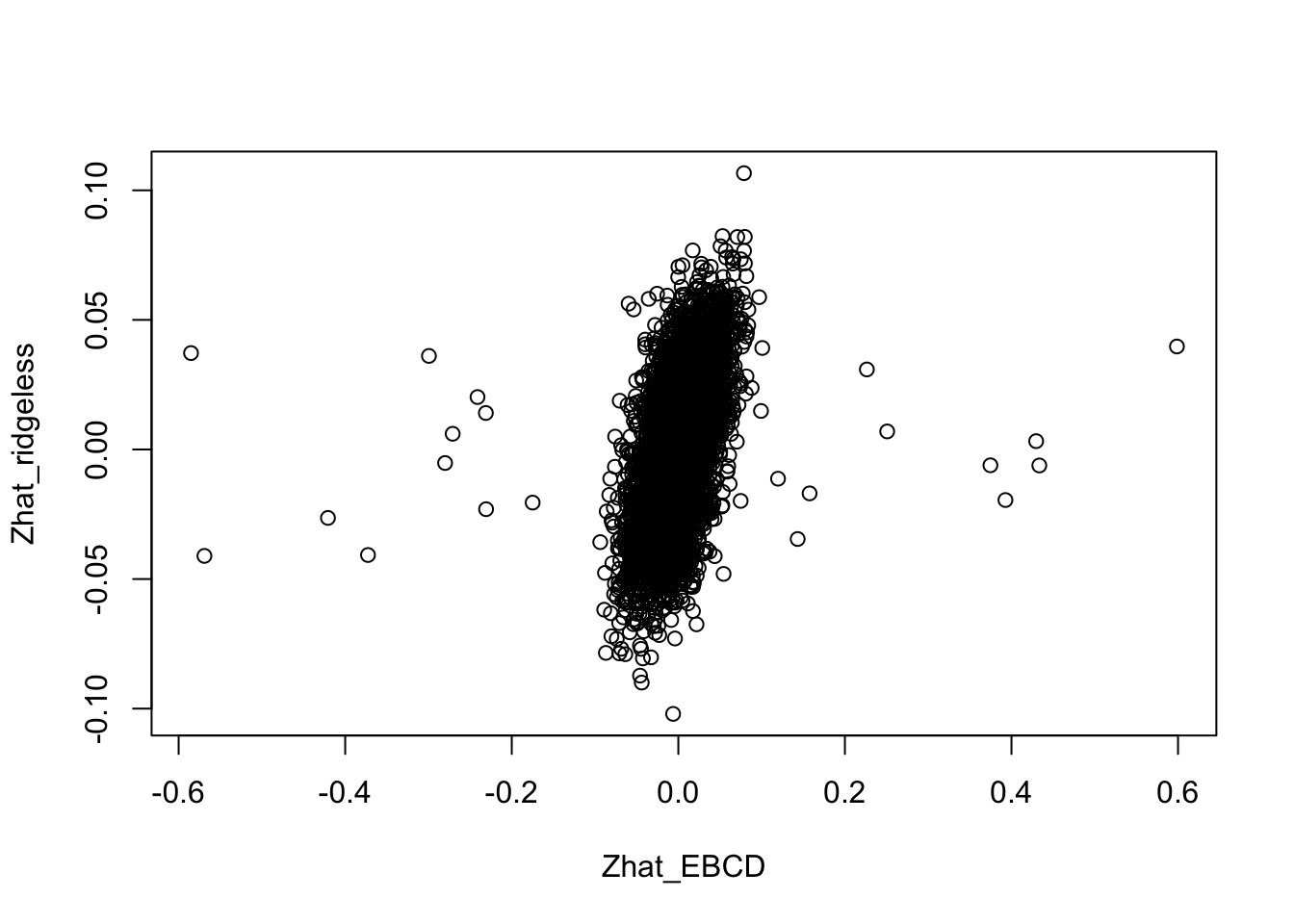

Past versions of unnamed-chunk-4-1.png

Version	Author	Date
7ee00c0	Matthew Stephens	2024-05-31

We can also orthogonalize the ridgeless solution:

plot(Zhat_EBCD,Polar.U(Zhat_ridgeless))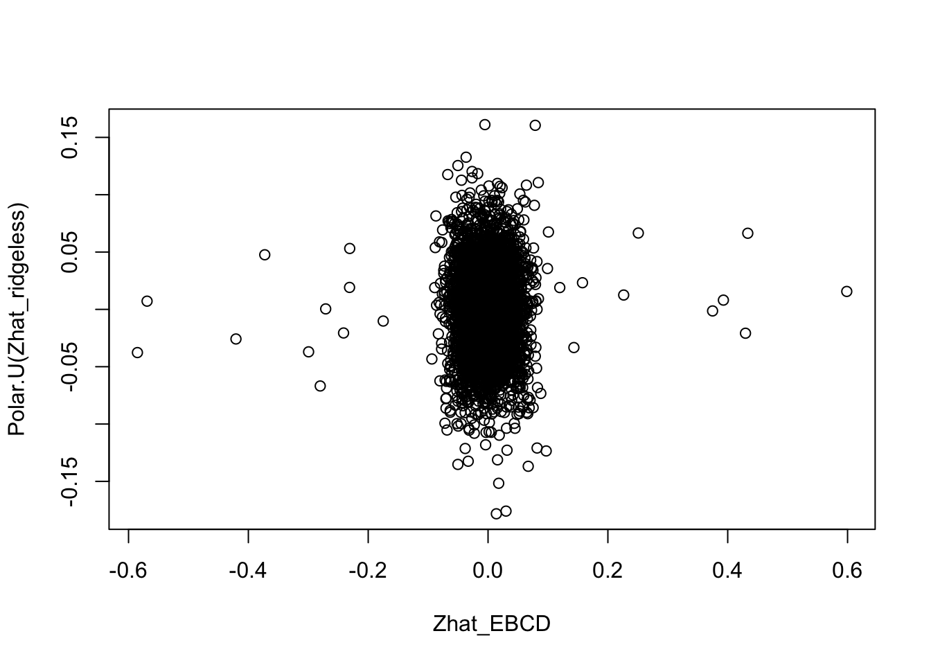

Past versions of unnamed-chunk-5-1.png

Version	Author	Date
7ee00c0	Matthew Stephens	2024-05-31

Comparison with true \(Z\)

Compare the estimates with the truth, it is clear that the orthogonal solutions are not as close to the truth as the (non-orthogonal) ridgeless solution.

plot(Z,Zhat_EBCD)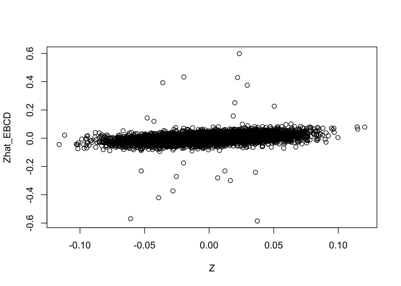

Past versions of unnamed-chunk-6-1.png

Version	Author	Date
7ee00c0	Matthew Stephens	2024-05-31

plot(Z,Zhat_ridgeless)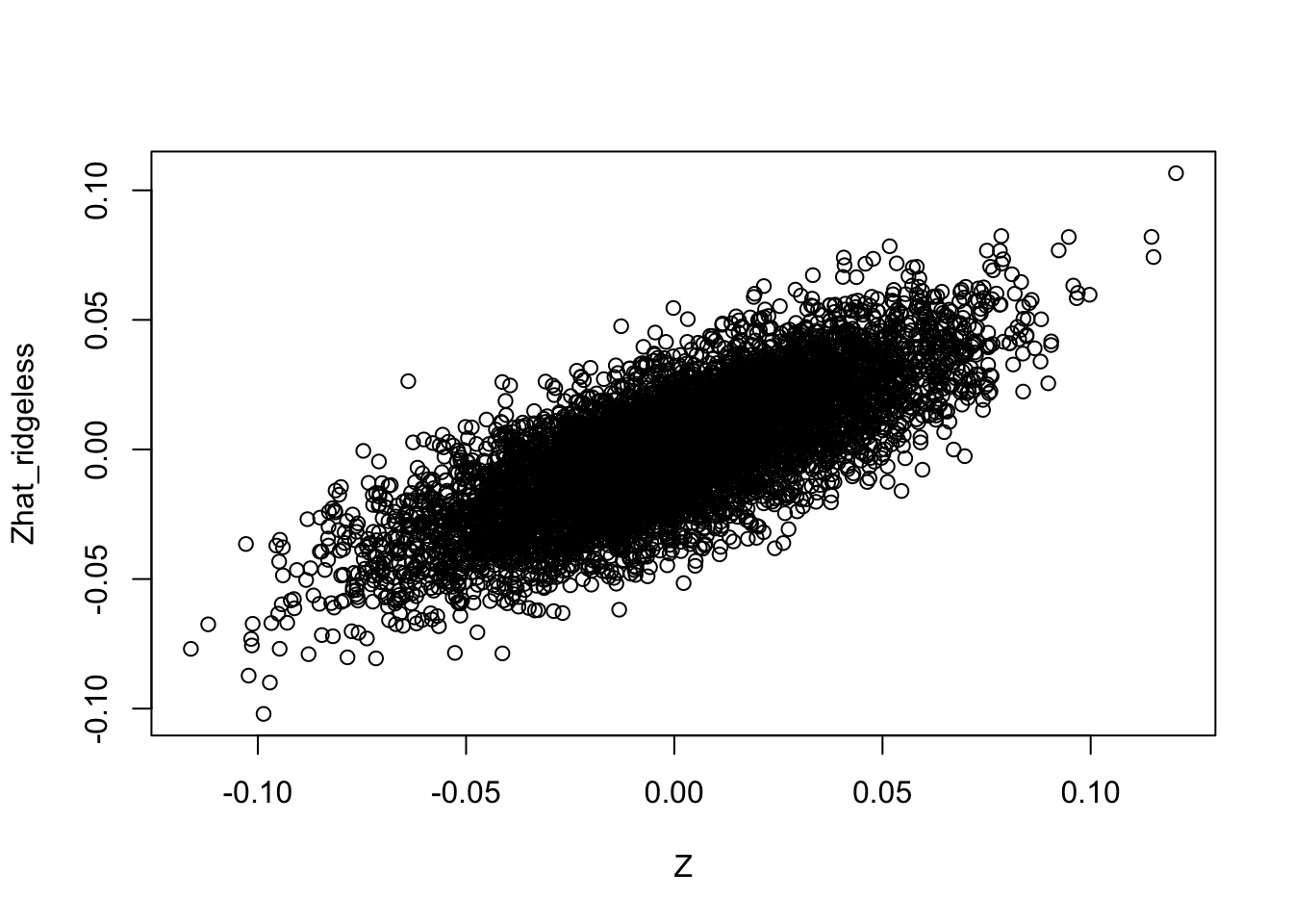

Past versions of unnamed-chunk-6-2.png

Version	Author	Date
7ee00c0	Matthew Stephens	2024-05-31

plot(Z,Polar.U(Zhat_ridgeless))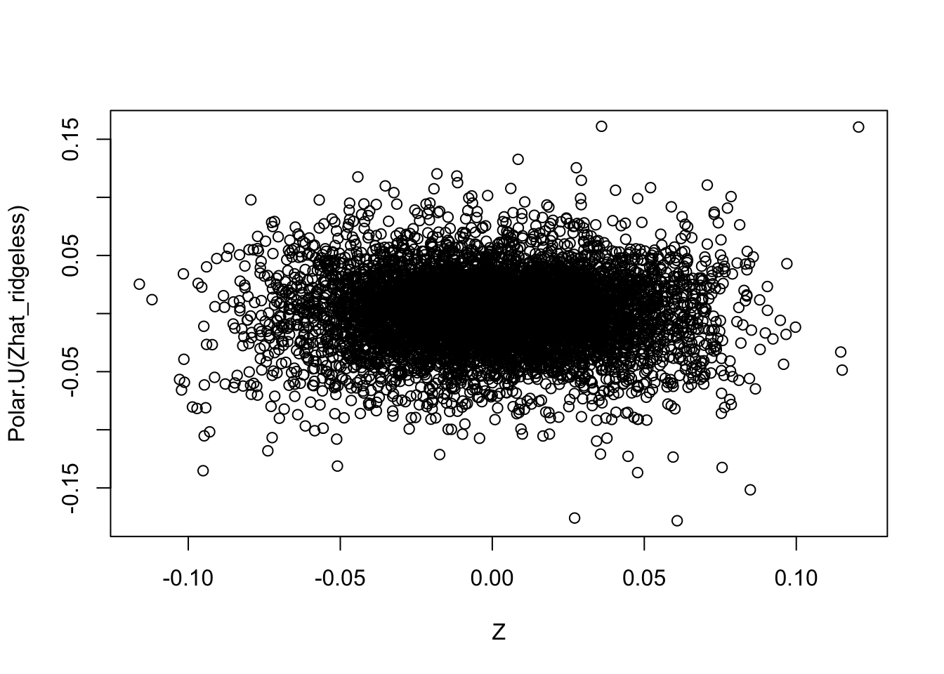

Past versions of unnamed-chunk-6-3.png

Version	Author	Date
7ee00c0	Matthew Stephens	2024-05-31

Estimates of \(L\) from estimated \(Z\)

The maximum likelihood estimate for \(L\) is \(X'Z(Z'Z)^-1\), or just \(X'Z\) for the case where \(Z\) is orthogonal. We can see that the estimates for \(L\) from these estimated \(Z\)s are very different from the true \(L\).

t(X) %*% Z # use true Z for comparison

         [,1]       [,2]          [,3]        [,4]        [,5]        [,6]
[1,] 1.102198 1.10431007  0.0880107137  1.11950583 -0.02735503 -0.08384765
[2,] 1.038237 1.09796987 -0.0004146382  0.04294618  0.94948187 -0.03021533
[3,] 1.103681 0.05696917  1.1431288765 -0.05428978 -0.15304383  0.96692646
[4,] 1.111669 0.06652107  1.0786249037  0.05591446 -0.10853902 -0.01437871
            [,7]
[1,]  0.04389647
[2,]  0.03182936
[3,] -0.07089470
[4,]  1.03156623

t(X) %*% Zhat_EBCD

          [,1]        [,2]       [,3]       [,4]       [,5]        [,6]
[1,] 1.3566380  0.92803423 -0.2214682  0.3190617 -0.1442323 -0.04998167
[2,] 1.4032931  0.09880374  0.2526351 -0.3216227  0.4427178  0.56912764
[3,] 0.9830229 -0.74304136 -0.1805494  0.2269756 -1.2014134  0.29403886
[4,] 0.4263371 -0.28631537  0.1855830 -0.2475666 -1.0533563 -0.03126267
          [,7]
[1,] 0.6709319
[2,] 0.6477064
[3,] 0.2851719
[4,] 1.3235760

t(X) %*% Polar.U(Zhat_ridgeless)

          [,1]       [,2]       [,3]        [,4]       [,5]        [,6]
[1,] 1.0383605 -0.7822616  0.5041554  0.84925740  0.5350675  0.58533737
[2,] 1.3584486 -0.6156229  0.3975160  0.06247522 -0.5333474  0.60876373
[3,] 0.2081658 -1.0274163 -0.5136721  0.05272136  0.4515585  0.46377117
[4,] 0.8533019 -0.2782730  0.1600512 -0.27963614  0.9778069 -0.05006597
           [,7]
[1,]  0.1776506
[2,] -0.2105689
[3,] -1.1954882
[4,] -1.1635612

The use of Zhat_ridgeless directly gives a good estimate of \(L\) (the MLE from Zhat_ridgeless gives essentially the exact answer, presumably because it is just inverting the process that gave Zhat_ridgeless).

t(X) %*% Zhat_ridgeless 

         [,1]         [,2]         [,3]       [,4]        [,5]         [,6]
[1,] 1.120804  1.087852095  0.032952219 1.11735591 -0.02950381 -0.047395883
[2,] 1.048871  1.055699202 -0.006828121 0.07458221  0.98111699 -0.034436371
[3,] 1.071945 -0.009974563  1.081919994 0.04438969 -0.05436426  1.059870056
[4,] 1.100219  0.034439539  1.065779114 0.09944643 -0.06500689  0.009917608
           [,7]
[1,] 0.08034810
[2,] 0.02760825
[3,] 0.02204994
[4,] 1.05586151

t(X) %*% Zhat_ridgeless %*% solve(t(Zhat_ridgeless) %*% Zhat_ridgeless + 1e-6*diag(7))

          [,1]          [,2]          [,3]          [,4]          [,5]
[1,] 0.9999992  9.999993e-01 -6.570554e-08  9.999997e-01 -4.046565e-07
[2,] 0.9999992  9.999993e-01 -1.021763e-07 -3.134373e-07  9.999996e-01
[3,] 0.9999992 -1.051062e-07  9.999993e-01 -8.284815e-09 -9.731525e-08
[4,] 0.9999992 -6.560003e-08  9.999993e-01  4.094909e-08 -1.071603e-07
              [,6]          [,7]
[1,] -8.891584e-08  2.252273e-08
[2,] -7.767085e-08 -2.531488e-08
[3,]  9.999997e-01 -3.621790e-07
[4,] -3.699679e-07  9.999997e-01

Session information

sessionInfo()

R version 4.2.1 (2022-06-23)
Platform: x86_64-apple-darwin17.0 (64-bit)
Running under: macOS Big Sur ... 10.16

Matrix products: default
BLAS:   /Library/Frameworks/R.framework/Versions/4.2/Resources/lib/libRblas.0.dylib
LAPACK: /Library/Frameworks/R.framework/Versions/4.2/Resources/lib/libRlapack.dylib

locale:
[1] en_US.UTF-8/en_US.UTF-8/en_US.UTF-8/C/en_US.UTF-8/en_US.UTF-8

attached base packages:
[1] stats     graphics  grDevices utils     datasets  methods   base     

loaded via a namespace (and not attached):
 [1] Rcpp_1.0.12       rstudioapi_0.15.0 whisker_0.4.1     knitr_1.45       
 [5] magrittr_2.0.3    workflowr_1.7.1   R6_2.5.1          rlang_1.1.2      
 [9] fastmap_1.1.1     fansi_1.0.6       highr_0.10        stringr_1.5.1    
[13] tools_4.2.1       xfun_0.41         utf8_1.2.4        cli_3.6.2        
[17] git2r_0.33.0      jquerylib_0.1.4   htmltools_0.5.7   rprojroot_2.0.4  
[21] yaml_2.3.8        digest_0.6.33     tibble_3.2.1      lifecycle_1.0.4  
[25] later_1.3.2       sass_0.4.8        vctrs_0.6.5       fs_1.6.3         
[29] promises_1.2.1    cachem_1.0.8      glue_1.6.2        evaluate_0.23    
[33] rmarkdown_2.25    stringi_1.8.3     bslib_0.6.1       compiler_4.2.1   
[37] pillar_1.9.0      jsonlite_1.8.8    httpuv_1.6.13     pkgconfig_2.0.3