ebpower
Matthew Stephens
2025-03-09
Last updated: 2025-03-20
Checks: 7 0
Knit directory: misc/analysis/
This reproducible R Markdown analysis was created with workflowr (version 1.7.1). The Checks tab describes the reproducibility checks that were applied when the results were created. The Past versions tab lists the development history.
Great! Since the R Markdown file has been committed to the Git repository, you know the exact version of the code that produced these results.
Great job! The global environment was empty. Objects defined in the global environment can affect the analysis in your R Markdown file in unknown ways. For reproduciblity it’s best to always run the code in an empty environment.
The command set.seed(1) was run prior to running the
code in the R Markdown file. Setting a seed ensures that any results
that rely on randomness, e.g. subsampling or permutations, are
reproducible.
Great job! Recording the operating system, R version, and package versions is critical for reproducibility.
Nice! There were no cached chunks for this analysis, so you can be confident that you successfully produced the results during this run.
Great job! Using relative paths to the files within your workflowr project makes it easier to run your code on other machines.
Great! You are using Git for version control. Tracking code development and connecting the code version to the results is critical for reproducibility.
The results in this page were generated with repository version 0c5ec0b. See the Past versions tab to see a history of the changes made to the R Markdown and HTML files.
Note that you need to be careful to ensure that all relevant files for
the analysis have been committed to Git prior to generating the results
(you can use wflow_publish or
wflow_git_commit). workflowr only checks the R Markdown
file, but you know if there are other scripts or data files that it
depends on. Below is the status of the Git repository when the results
were generated:
Ignored files:
    Ignored:    .DS_Store
    Ignored:    .Rhistory
    Ignored:    .Rproj.user/
    Ignored:    analysis/.RData
    Ignored:    analysis/.Rhistory
    Ignored:    analysis/ALStruct_cache/
    Ignored:    data/.Rhistory
    Ignored:    data/methylation-data-for-matthew.rds
    Ignored:    data/pbmc/
    Ignored:    data/pbmc_purified.RData

Untracked files:
    Untracked:  .dropbox
    Untracked:  Icon
    Untracked:  analysis/GHstan.Rmd
    Untracked:  analysis/GTEX-cogaps.Rmd
    Untracked:  analysis/PACS.Rmd
    Untracked:  analysis/Rplot.png
    Untracked:  analysis/SPCAvRP.rmd
    Untracked:  analysis/abf_comparisons.Rmd
    Untracked:  analysis/admm_02.Rmd
    Untracked:  analysis/admm_03.Rmd
    Untracked:  analysis/bispca.Rmd
    Untracked:  analysis/cache/
    Untracked:  analysis/cholesky.Rmd
    Untracked:  analysis/compare-transformed-models.Rmd
    Untracked:  analysis/cormotif.Rmd
    Untracked:  analysis/cp_ash.Rmd
    Untracked:  analysis/eQTL.perm.rand.pdf
    Untracked:  analysis/eb_prepilot.Rmd
    Untracked:  analysis/eb_snmu.Rmd
    Untracked:  analysis/eb_var.Rmd
    Untracked:  analysis/ebpmf1.Rmd
    Untracked:  analysis/ebpmf_sla_text.Rmd
    Untracked:  analysis/ebspca_sims.Rmd
    Untracked:  analysis/explore_psvd.Rmd
    Untracked:  analysis/fa_check_identify.Rmd
    Untracked:  analysis/fa_iterative.Rmd
    Untracked:  analysis/flash_cov_overlapping_groups_init.Rmd
    Untracked:  analysis/flash_test_tree.Rmd
    Untracked:  analysis/flashier_newgroups.Rmd
    Untracked:  analysis/flashier_nmf_triples.Rmd
    Untracked:  analysis/flashier_pbmc.Rmd
    Untracked:  analysis/flashier_snn_shifted_prior.Rmd
    Untracked:  analysis/greedy_ebpmf_exploration_00.Rmd
    Untracked:  analysis/ieQTL.perm.rand.pdf
    Untracked:  analysis/lasso_em_03.Rmd
    Untracked:  analysis/m6amash.Rmd
    Untracked:  analysis/mash_bhat_z.Rmd
    Untracked:  analysis/mash_ieqtl_permutations.Rmd
    Untracked:  analysis/methylation_example.Rmd
    Untracked:  analysis/mixsqp.Rmd
    Untracked:  analysis/mr.ash_lasso_init.Rmd
    Untracked:  analysis/mr.mash.test.Rmd
    Untracked:  analysis/mr_ash_modular.Rmd
    Untracked:  analysis/mr_ash_parameterization.Rmd
    Untracked:  analysis/mr_ash_ridge.Rmd
    Untracked:  analysis/mv_gaussian_message_passing.Rmd
    Untracked:  analysis/nejm.Rmd
    Untracked:  analysis/nmf_bg.Rmd
    Untracked:  analysis/nonneg_underapprox.Rmd
    Untracked:  analysis/normal_conditional_on_r2.Rmd
    Untracked:  analysis/normalize.Rmd
    Untracked:  analysis/pbmc.Rmd
    Untracked:  analysis/pca_binary_weighted.Rmd
    Untracked:  analysis/pca_l1.Rmd
    Untracked:  analysis/poisson_nmf_approx.Rmd
    Untracked:  analysis/poisson_shrink.Rmd
    Untracked:  analysis/poisson_transform.Rmd
    Untracked:  analysis/qrnotes.txt
    Untracked:  analysis/ridge_iterative_02.Rmd
    Untracked:  analysis/ridge_iterative_splitting.Rmd
    Untracked:  analysis/samps/
    Untracked:  analysis/sc_bimodal.Rmd
    Untracked:  analysis/shrinkage_comparisons_changepoints.Rmd
    Untracked:  analysis/susie_cov.Rmd
    Untracked:  analysis/susie_en.Rmd
    Untracked:  analysis/susie_z_investigate.Rmd
    Untracked:  analysis/svd-timing.Rmd
    Untracked:  analysis/temp.RDS
    Untracked:  analysis/temp.Rmd
    Untracked:  analysis/test-figure/
    Untracked:  analysis/test.Rmd
    Untracked:  analysis/test.Rpres
    Untracked:  analysis/test.md
    Untracked:  analysis/test_qr.R
    Untracked:  analysis/test_sparse.Rmd
    Untracked:  analysis/tree_dist_top_eigenvector.Rmd
    Untracked:  analysis/z.txt
    Untracked:  code/multivariate_testfuncs.R
    Untracked:  code/rqb.hacked.R
    Untracked:  data/4matthew/
    Untracked:  data/4matthew2/
    Untracked:  data/E-MTAB-2805.processed.1/
    Untracked:  data/ENSG00000156738.Sim_Y2.RDS
    Untracked:  data/GDS5363_full.soft.gz
    Untracked:  data/GSE41265_allGenesTPM.txt
    Untracked:  data/Muscle_Skeletal.ACTN3.pm1Mb.RDS
    Untracked:  data/P.rds
    Untracked:  data/Thyroid.FMO2.pm1Mb.RDS
    Untracked:  data/bmass.HaemgenRBC2016.MAF01.Vs2.MergedDataSources.200kRanSubset.ChrBPMAFMarkerZScores.vs1.txt.gz
    Untracked:  data/bmass.HaemgenRBC2016.Vs2.NewSNPs.ZScores.hclust.vs1.txt
    Untracked:  data/bmass.HaemgenRBC2016.Vs2.PreviousSNPs.ZScores.hclust.vs1.txt
    Untracked:  data/eb_prepilot/
    Untracked:  data/finemap_data/fmo2.sim/b.txt
    Untracked:  data/finemap_data/fmo2.sim/dap_out.txt
    Untracked:  data/finemap_data/fmo2.sim/dap_out2.txt
    Untracked:  data/finemap_data/fmo2.sim/dap_out2_snp.txt
    Untracked:  data/finemap_data/fmo2.sim/dap_out_snp.txt
    Untracked:  data/finemap_data/fmo2.sim/data
    Untracked:  data/finemap_data/fmo2.sim/fmo2.sim.config
    Untracked:  data/finemap_data/fmo2.sim/fmo2.sim.k
    Untracked:  data/finemap_data/fmo2.sim/fmo2.sim.k4.config
    Untracked:  data/finemap_data/fmo2.sim/fmo2.sim.k4.snp
    Untracked:  data/finemap_data/fmo2.sim/fmo2.sim.ld
    Untracked:  data/finemap_data/fmo2.sim/fmo2.sim.snp
    Untracked:  data/finemap_data/fmo2.sim/fmo2.sim.z
    Untracked:  data/finemap_data/fmo2.sim/pos.txt
    Untracked:  data/logm.csv
    Untracked:  data/m.cd.RDS
    Untracked:  data/m.cdu.old.RDS
    Untracked:  data/m.new.cd.RDS
    Untracked:  data/m.old.cd.RDS
    Untracked:  data/mainbib.bib.old
    Untracked:  data/mat.csv
    Untracked:  data/mat.txt
    Untracked:  data/mat_new.csv
    Untracked:  data/matrix_lik.rds
    Untracked:  data/paintor_data/
    Untracked:  data/running_data_chris.csv
    Untracked:  data/running_data_matthew.csv
    Untracked:  data/temp.txt
    Untracked:  data/y.txt
    Untracked:  data/y_f.txt
    Untracked:  data/zscore_jointLCLs_m6AQTLs_susie_eQTLpruned.rds
    Untracked:  data/zscore_jointLCLs_random.rds
    Untracked:  explore_udi.R
    Untracked:  output/fit.k10.rds
    Untracked:  output/fit.nn.pbmc.purified.rds
    Untracked:  output/fit.nn.rds
    Untracked:  output/fit.nn.s.001.rds
    Untracked:  output/fit.nn.s.01.rds
    Untracked:  output/fit.nn.s.1.rds
    Untracked:  output/fit.nn.s.10.rds
    Untracked:  output/fit.snn.s.001.rds
    Untracked:  output/fit.snn.s.01.nninit.rds
    Untracked:  output/fit.snn.s.01.rds
    Untracked:  output/fit.varbvs.RDS
    Untracked:  output/fit2.nn.pbmc.purified.rds
    Untracked:  output/glmnet.fit.RDS
    Untracked:  output/snn07.txt
    Untracked:  output/snn34.txt
    Untracked:  output/test.bv.txt
    Untracked:  output/test.gamma.txt
    Untracked:  output/test.hyp.txt
    Untracked:  output/test.log.txt
    Untracked:  output/test.param.txt
    Untracked:  output/test2.bv.txt
    Untracked:  output/test2.gamma.txt
    Untracked:  output/test2.hyp.txt
    Untracked:  output/test2.log.txt
    Untracked:  output/test2.param.txt
    Untracked:  output/test3.bv.txt
    Untracked:  output/test3.gamma.txt
    Untracked:  output/test3.hyp.txt
    Untracked:  output/test3.log.txt
    Untracked:  output/test3.param.txt
    Untracked:  output/test4.bv.txt
    Untracked:  output/test4.gamma.txt
    Untracked:  output/test4.hyp.txt
    Untracked:  output/test4.log.txt
    Untracked:  output/test4.param.txt
    Untracked:  output/test5.bv.txt
    Untracked:  output/test5.gamma.txt
    Untracked:  output/test5.hyp.txt
    Untracked:  output/test5.log.txt
    Untracked:  output/test5.param.txt

Unstaged changes:
    Modified:   .gitignore
    Modified:   analysis/ebnm_binormal.Rmd
    Modified:   analysis/flashier_log1p.Rmd
    Modified:   analysis/flashier_sla_text.Rmd
    Modified:   analysis/logistic_z_scores.Rmd
    Modified:   analysis/mr_ash_pen.Rmd
    Modified:   analysis/nmu_em.Rmd
    Modified:   analysis/susie_flash.Rmd
    Modified:   misc.Rproj
Note that any generated files, e.g. HTML, png, CSS, etc., are not included in this status report because it is ok for generated content to have uncommitted changes.
These are the previous versions of the repository in which changes were
made to the R Markdown (analysis/ebpower.Rmd) and HTML
(docs/ebpower.html) files. If you’ve configured a remote
Git repository (see ?wflow_git_remote), click on the
hyperlinks in the table below to view the files as they were in that
past version.
| File | Version | Author | Date | Message |
|---|---|---|---|---|
| Rmd | 0c5ec0b | Matthew Stephens | 2025-03-20 | workflowr::wflow_publish("ebpower.Rmd") |
| html | b396544 | Matthew Stephens | 2025-03-16 | Build site. |
| Rmd | fe667eb | Matthew Stephens | 2025-03-16 | workflowr::wflow_publish("ebpower.Rmd") |
| html | 9006efb | Matthew Stephens | 2025-03-15 | Build site. |
| Rmd | 4c2850b | Matthew Stephens | 2025-03-15 | workflowr::wflow_publish("ebpower.Rmd") |
| html | 7c17b31 | Matthew Stephens | 2025-03-15 | Build site. |
| Rmd | 0608521 | Matthew Stephens | 2025-03-15 | workflowr::wflow_publish("ebpower.Rmd") |
| html | 2956a39 | Matthew Stephens | 2025-03-12 | Build site. |
| Rmd | 6aa4dfe | Matthew Stephens | 2025-03-12 | workflowr::wflow_publish("analysis/ebpower.Rmd") |
# load the ebnm library and define an ebnm_binormal function

library("ebnm")

dbinormal = function (x,s,s0,lambda,log=TRUE){
  pi0 = 0.5
  pi1 = 0.5
  s2 = s^2
  s02 = s0^2
  l0 = dnorm(x,0,sqrt(lambda^2 * s02 + s2),log=TRUE)
  l1 = dnorm(x,lambda,sqrt(lambda^2 * s02 + s2),log=TRUE)
  logsum = log(pi0*exp(l0) + pi1*exp(l1))

  m = pmax(l0,l1)
  logsum = m + log(pi0*exp(l0-m) + pi1*exp(l1-m))
  if (log) return(sum(logsum))
  else return(exp(sum(logsum)))
}

ebnm_binormal = function(x,s){
  x = drop(x)
  s0 = 0.01
  lambda = optimize(function(lambda){-dbinormal(x,s,s0,lambda,log=TRUE)},
              lower = 0, upper = max(x))$minimum
  g = ashr::normalmix(pi=c(0.5,0.5), mean=c(0,lambda), sd=c(lambda * s0,lambda * s0))
  postmean = ashr::postmean(g,ashr::set_data(x,s))
  postsd = ashr::postsd(g,ashr::set_data(x,s))
  return(list(g = g, posterior = data.frame(mean=postmean,sd=postsd)))
}
Introduction
I want to implement an EB version of the power update for a symmetric data matrix S.
Rank 1
These are the update functions for the regular power update and the EB version.
# This is just the regular power update, used for initialization
power_update_r1 = function(S,v){
  newv = drop(S %*% v)
  if(!all(newv==0))
    v = newv/sqrt(sum(newv^2))
  return(v)
}

eb_power_update_r1 = function(S,v,ebnm_fn,sigma){
  newv = drop(S %*% v)
  if(!all(newv==0))
    v = ebnm_fn(newv, sigma)$posterior$mean
  if(!all(v==0))
    v = v/sqrt(sum(v^2))
  return(v)
}
Non-overlapping equal group
First I simulate data under non-overlapping equal groups, so the
matrix is essentially a noisy version of a (block) identity matrix. I
set up x here to be the 6 factors of a hierarchical tree
structure for later use, but I only use the bottom 4 factors so it is
not actually a tree.
set.seed(1)
n = 40
x = cbind(c(rep(1,n),rep(0,n)), c(rep(0,n),rep(1,n)), c(rep(1,n/2),rep(0,3*n/2)), c(rep(0,n/2), rep(1,n/2), rep(0,n)), c(rep(0,n),rep(1,n/2),rep(0,n/2)), c(rep(0,3*n/2),rep(1,n/2)))
E = matrix(0.1*rnorm(2*n*2*n),nrow=2*n)
E = E+t(E) #symmetric errors
S = x %*% diag(c(0,0,1,1,1,1)) %*% t(x) + E
image(S)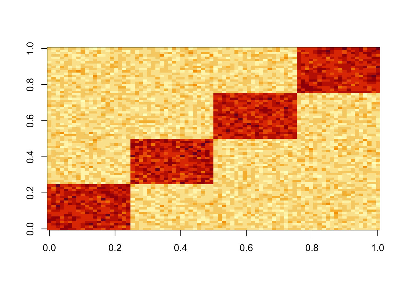
The first four PCs all have almost the same eigenvalues here. The first PC is piecewise constant on the four groups, with essentially arbitrary values on each group.
S.svd = svd(S)
S.svd$d[1:10]
[1] 20.319342 20.190306 19.925768 19.825598 2.444629 2.396738 2.310219
[8] 2.234729 2.179483 2.153417pc1 = S.svd$v[,1]
plot(pc1)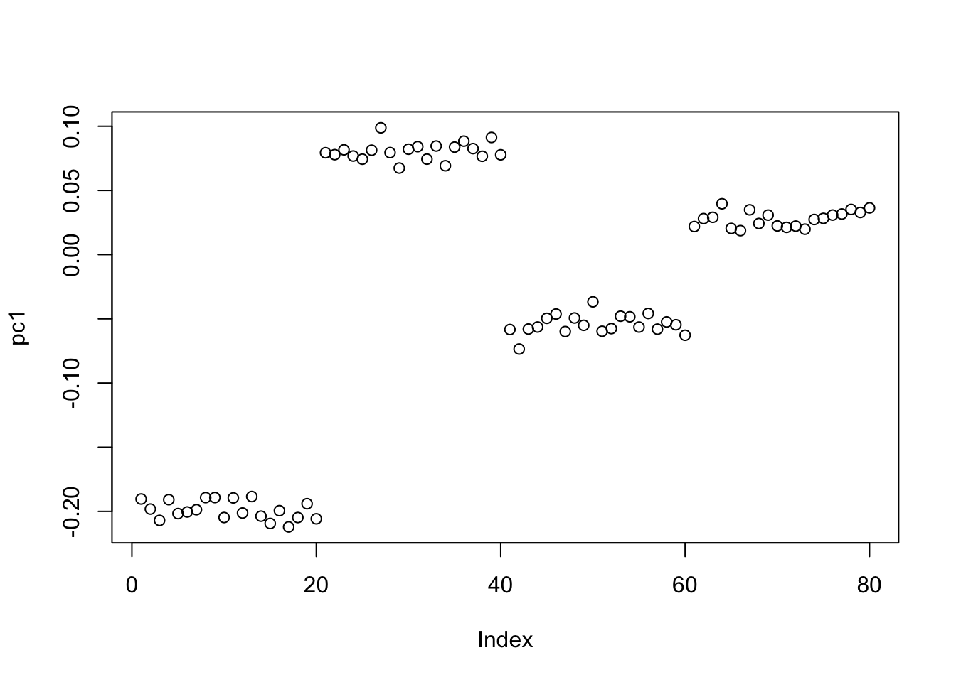
Point Laplace
Power update with point laplace: it finds one of the groups.
v = pc1
for(i in 1:100)
  v = eb_power_update_r1(S, v, ebnm_point_laplace, sqrt(mean(S^2)))
plot(v, ylim=c(-0.25,0.25))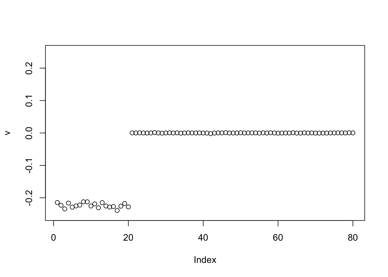
I expected that it could find a solution with both positive and negative values (two different groups) if initialized differently. So I tried initilializing it like that, but it still found just one group.
v = c(rep(1,n/2),rep(-1,n/2),rep(0,n))
v = v/sqrt(sum(v^2))
for(i in 1:10){
  v = eb_power_update_r1(S, v, ebnm_point_laplace, sqrt(mean(S^2)))
}
plot(v, ylim=c(-0.25,0.25))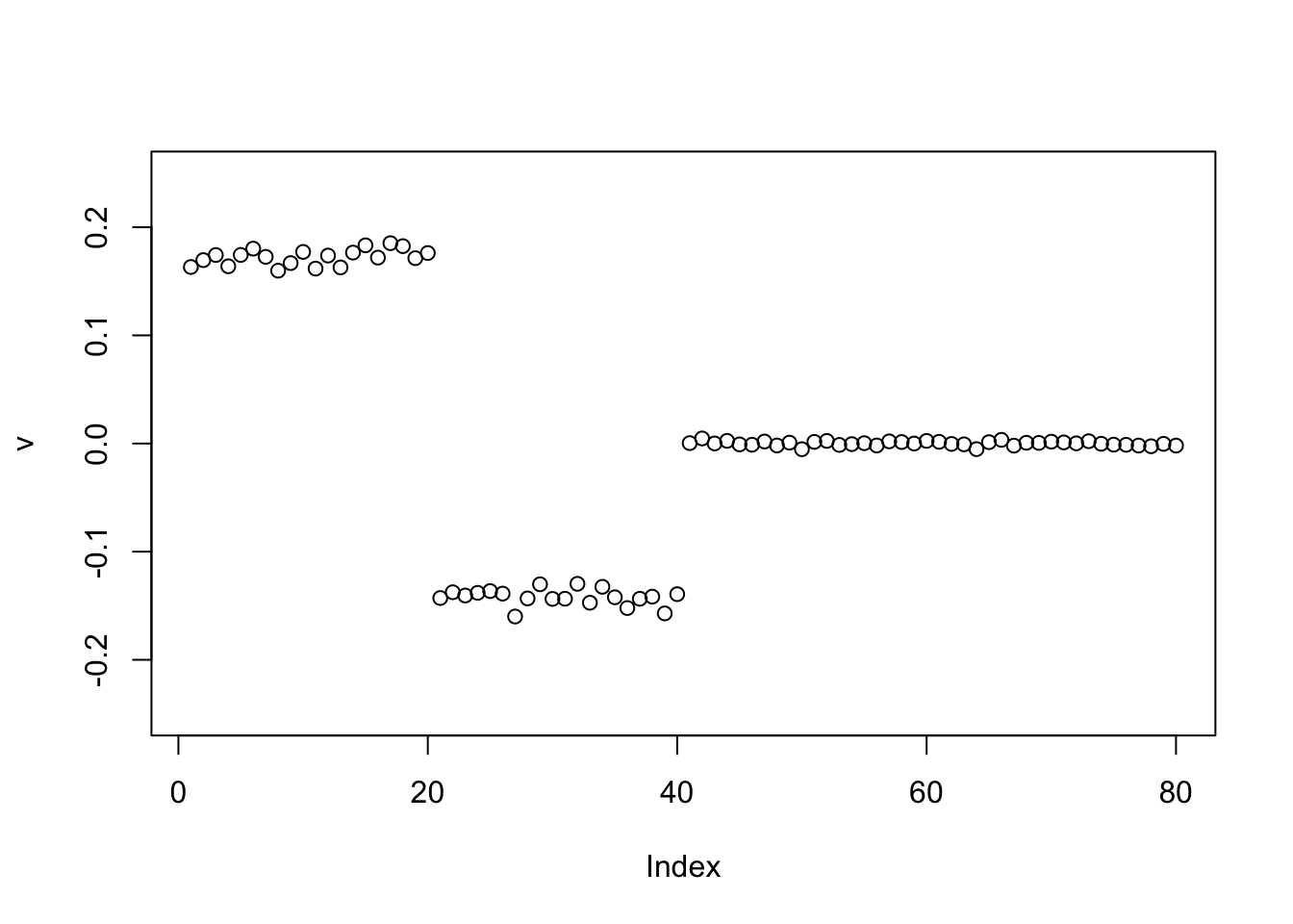
Try a different one:
v = c(rep(0,n/2),rep(1,n/2),rep(-1,n/2),rep(0,n/2))
v = v/sqrt(sum(v^2))
for(i in 1:100){
  v = eb_power_update_r1(S, v, ebnm_point_laplace, sqrt(mean(S^2)))
}
plot(v, ylim=c(-0.25,0.25))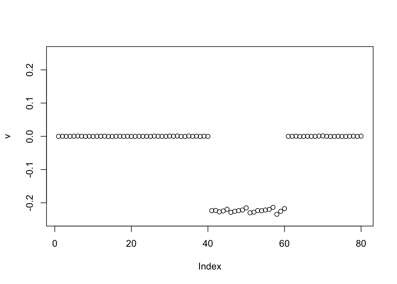
And again.. It seems to consistently want to find one group. I was a bit surprised by this, but I guess having just one group allows it to have a sparser solution, and this is winning out here.
v = c(rep(1,n/2),rep(0,n/2),rep(-1,n/2),rep(0,n/2))
v = v/sqrt(sum(v^2))
for(i in 1:100){
  v = eb_power_update_r1(S, v, ebnm_point_laplace, sqrt(mean(S^2)))
}
plot(v, ylim=c(-0.25,0.25))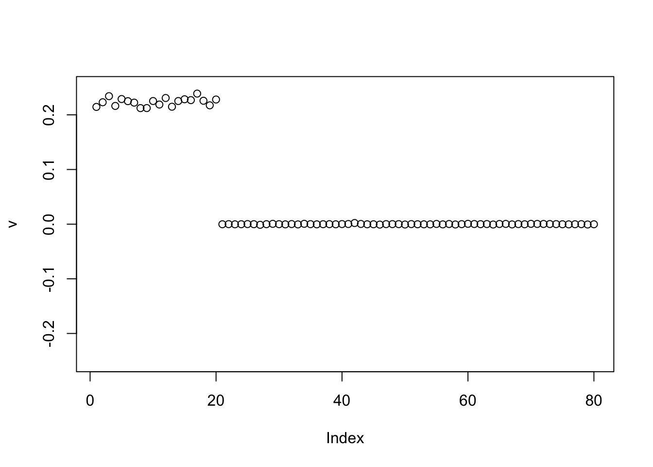
Point Exponential
Power update with point exponential: it finds one of the groups, as I expected.
v = pc1
for(i in 1:100){
  v = eb_power_update_r1(S, v, ebnm_point_exponential, sqrt(mean(S^2)))
}
plot(v, ylim=c(-0.25,0.25))
Here I initialize with the negative of the first PC, and it finds a single group again. Again I expected this.
v = -pc1
for(i in 1:100){
  v = eb_power_update_r1(S, v, ebnm_point_exponential, sqrt(mean(S^2)))
}
plot(v, ylim=c(-0.25,0.25))
Binormal prior
Try binormal prior; this behaves as expected.
v = pc1
for(i in 1:100){
  v = eb_power_update_r1(S, v, ebnm_binormal, sqrt(mean(S^2)))
}
plot(v, ylim=c(-0.25,0.25))
However, when I try initializing with the negative of the first PC, it finds two groups. This was unexpected to me, but it makes sense in retrospect, especially as I fix the sparsity of the binormal prior to have 0.5 mass on the 0 component. Also, it is easier for the point exponential to move to sparser solutions because it is unimodal at 0. Possibly it supports the idea of running the point exponential prior before running binormal.
v = -pc1
for(i in 1:100){
  v = eb_power_update_r1(S, v, ebnm_binormal, sqrt(mean(S^2)))
}
plot(v, ylim=c(-0.25,0.25))
Here is the same thing running point exponential before binormal.
v = -pc1
for(i in 1:100){
  v = eb_power_update_r1(S, v, ebnm_point_exponential, sqrt(mean(S^2)))
}
for(i in 1:100){
  v = eb_power_update_r1(S, v, ebnm_binormal, sqrt(mean(S^2)))
}
plot(v, ylim=c(-0.25,0.25))
Generalized Binary
The GB behaves like the binormal prior:
v = pc1
for(i in 1:100){
  v = eb_power_update_r1(S, v, ebnm_generalized_binary, sqrt(mean(S^2)))
}
plot(v, ylim=c(-0.25,0.25))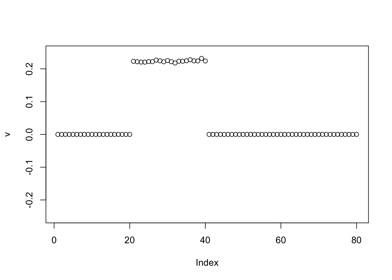
Interestingly, in this example the GB prior also converges to the 2 group solution when initialized from the negative of the first PC.
v = -pc1
for(i in 1:100){
  v = eb_power_update_r1(S, v, ebnm_generalized_binary, sqrt(mean(S^2)))
}
plot(v, ylim=c(-0.25,0.25))
Non-overlapping equal group II - centered
I reran the above after centering the matrix to see how this affects things. I expected it would change the point laplace to find some +-1 solutions, but others should maybe not change much.
S = S-mean(S)Now it is the top 3 PCs that have almost the same eigenvalues, as I have effectively removed one of them. The first PC is still piecewise constant on the four groups, with essentially arbitrary values on each group.
S.svd = svd(S)
S.svd$d[1:10]
[1] 20.286102 20.151260 19.855386 2.447533 2.404582 2.312658 2.263692
[8] 2.199055 2.160337 2.091697pc1 = S.svd$v[,1]
plot(pc1)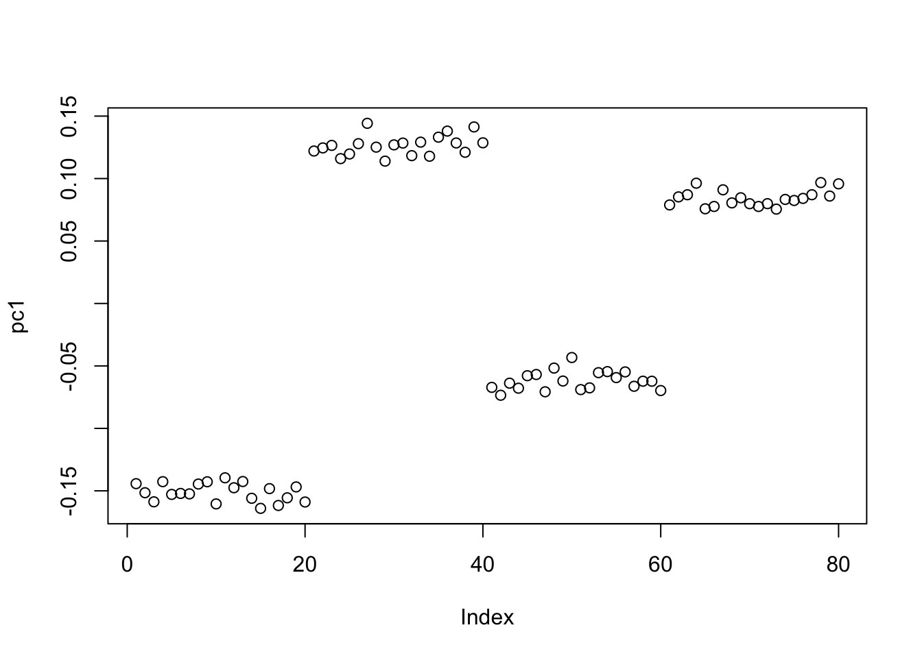
Point Laplace
Point laplace now finds a +-1 solution as I expected.
v = pc1
for(i in 1:100)
  v = eb_power_update_r1(S, v, ebnm_point_laplace, sqrt(mean(S^2)))
plot(v, ylim=c(-0.25,0.25))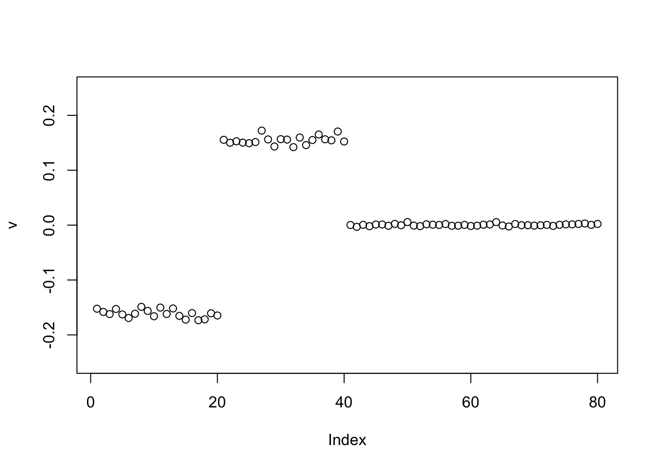
Point Exponential
Point exponential finds one group, as I expected.
v = pc1
for(i in 1:100){
  v = eb_power_update_r1(S, v, ebnm_point_exponential, sqrt(mean(S^2)))
}
plot(v, ylim=c(-0.25,0.25))
| Version | Author | Date |
|---|---|---|
| b396544 | Matthew Stephens | 2025-03-16 |
Here I initialize with the negative of the first PC, and it finds a single group again. Again I expected this.
v = -pc1
for(i in 1:100){
  v = eb_power_update_r1(S, v, ebnm_point_exponential, sqrt(mean(S^2)))
}
plot(v, ylim=c(-0.25,0.25))
Binormal prior
The binormal prior behaves just as before centering:
v = pc1
for(i in 1:100){
  v = eb_power_update_r1(S, v, ebnm_binormal, sqrt(mean(S^2)))
}
plot(v, ylim=c(-0.25,0.25))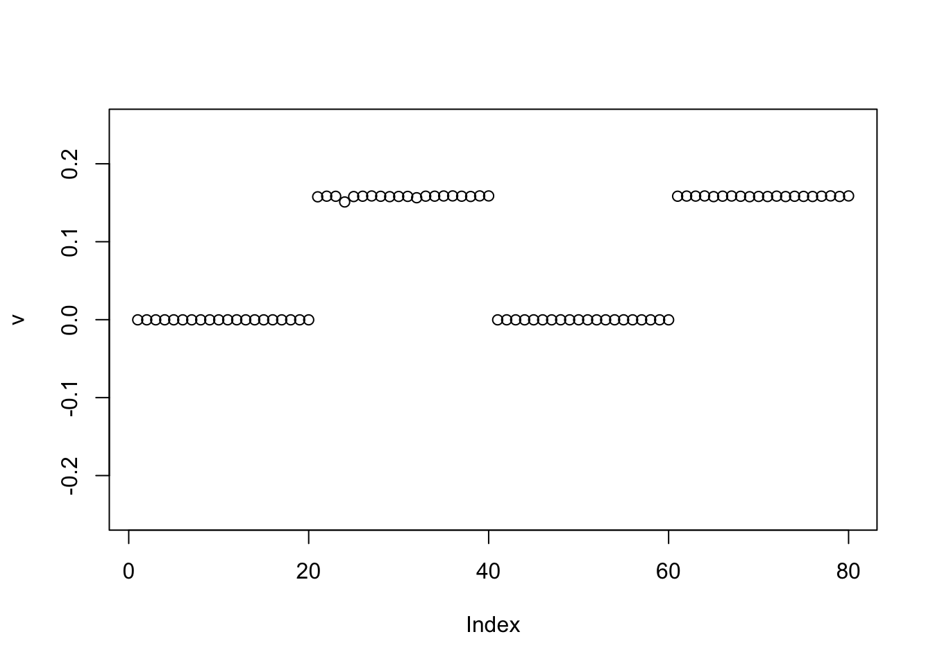
v = -pc1
for(i in 1:100){
  v = eb_power_update_r1(S, v, ebnm_binormal, sqrt(mean(S^2)))
}
plot(v, ylim=c(-0.25,0.25))
Generalized Binary
The GB also behaves the same as without centering
v = pc1
for(i in 1:100){
  v = eb_power_update_r1(S, v, ebnm_generalized_binary, sqrt(mean(S^2)))
}
plot(v, ylim=c(-0.25,0.25))
v = -pc1
for(i in 1:100){
  v = eb_power_update_r1(S, v, ebnm_generalized_binary, sqrt(mean(S^2)))
}
plot(v, ylim=c(-0.25,0.25))
Tree model
Simulate data under a tree model
set.seed(1)
S = x %*% diag(c(1,1,1,1,1,1)) %*% t(x) + E
image(S)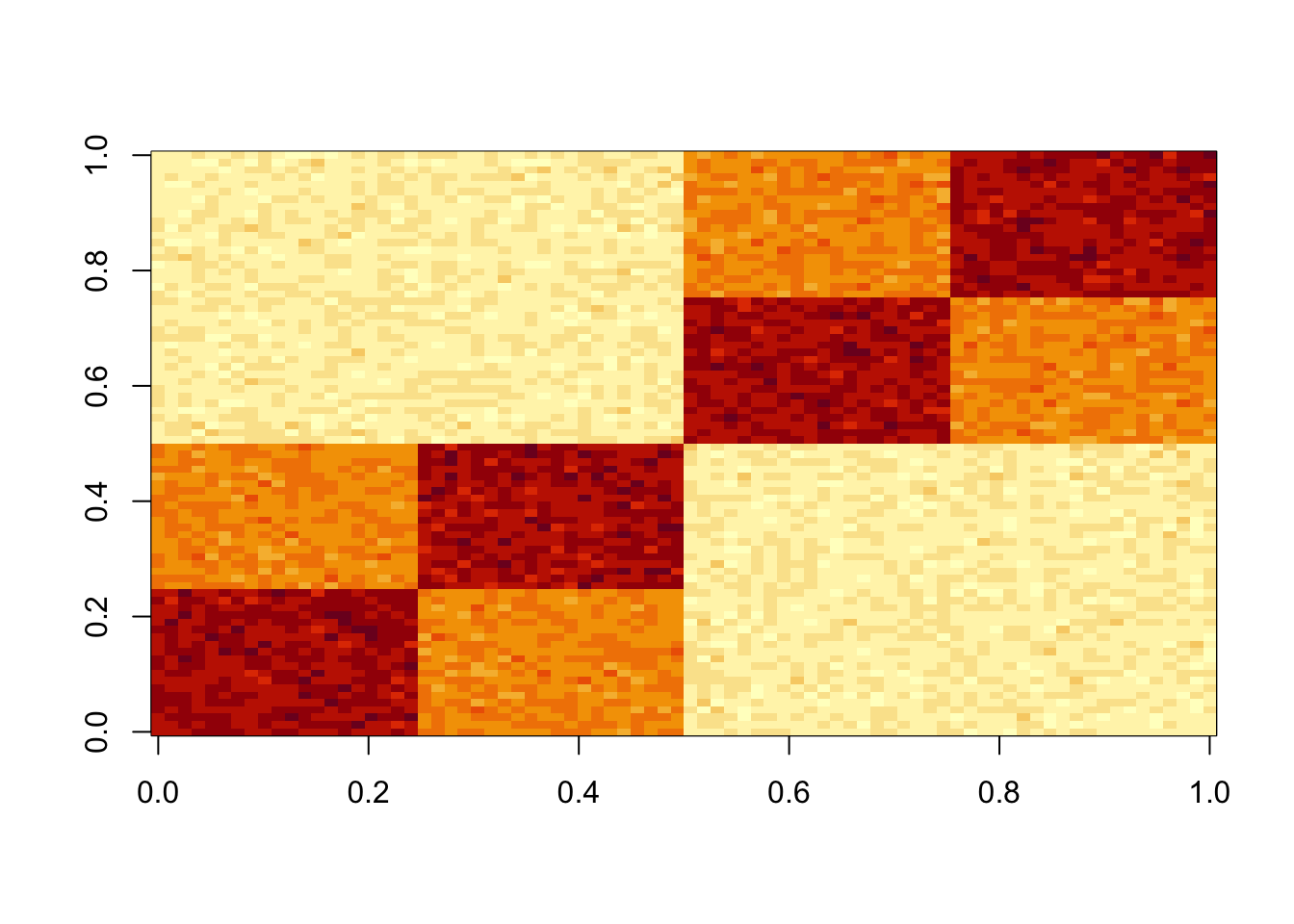
Check the PCs. The top 2 PCs have similar eigenvalues. The first one splits the top two branches; the second one also splits them, but is almost constant.
S.svd = svd(S)
S.svd$d[1:10]
[1] 59.965607 59.885902 20.283062 20.024521 2.444106 2.397191 2.310779
[8] 2.232964 2.180340 2.154132pc1 = cbind(S.svd$v[,1])
pc2 = cbind(S.svd$v[,2])
plot(pc1,ylim=c(-0.25,0.25))
abline(h=0)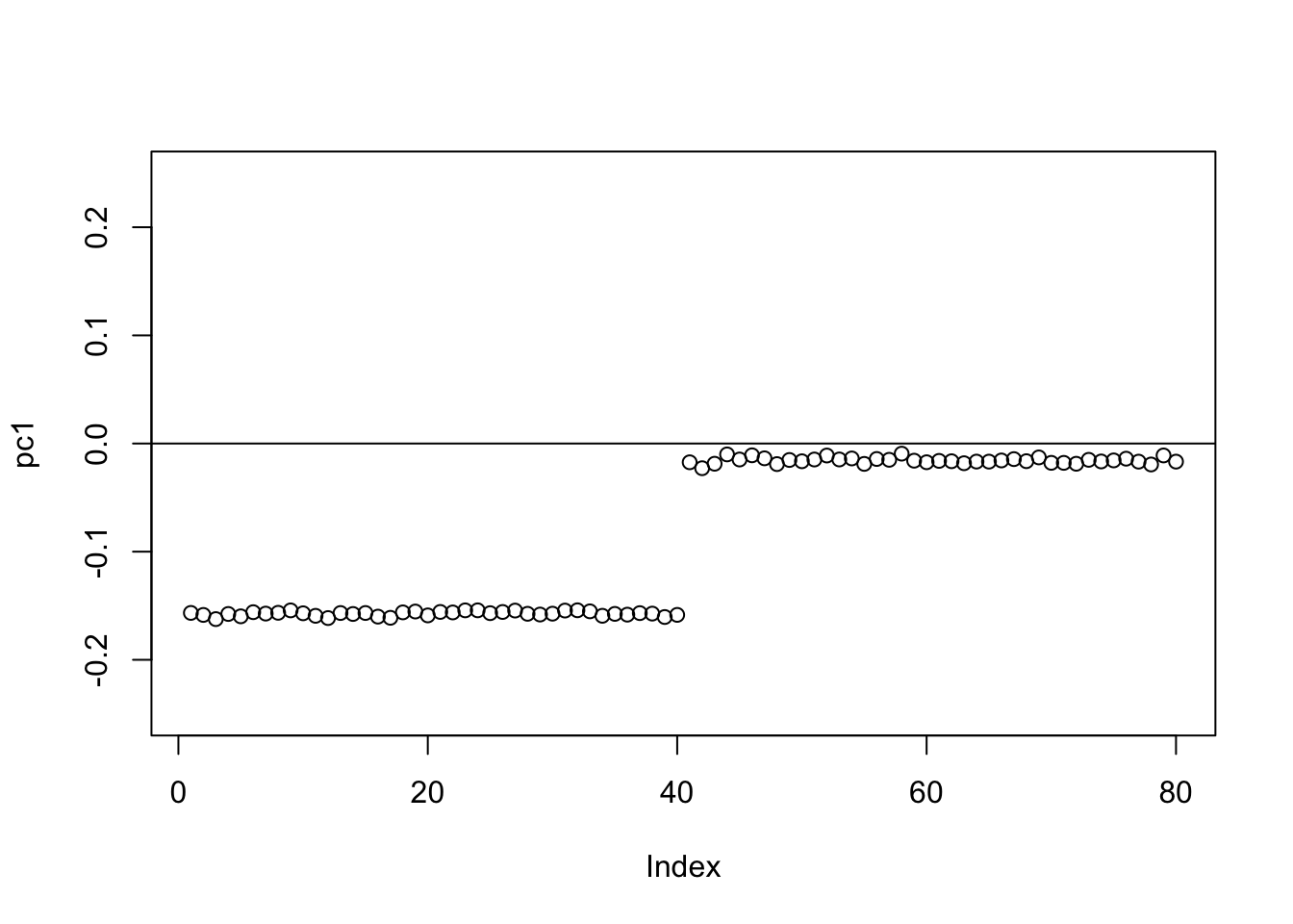
plot(pc2,ylim=c(-0.25,0.25))
abline(h=0)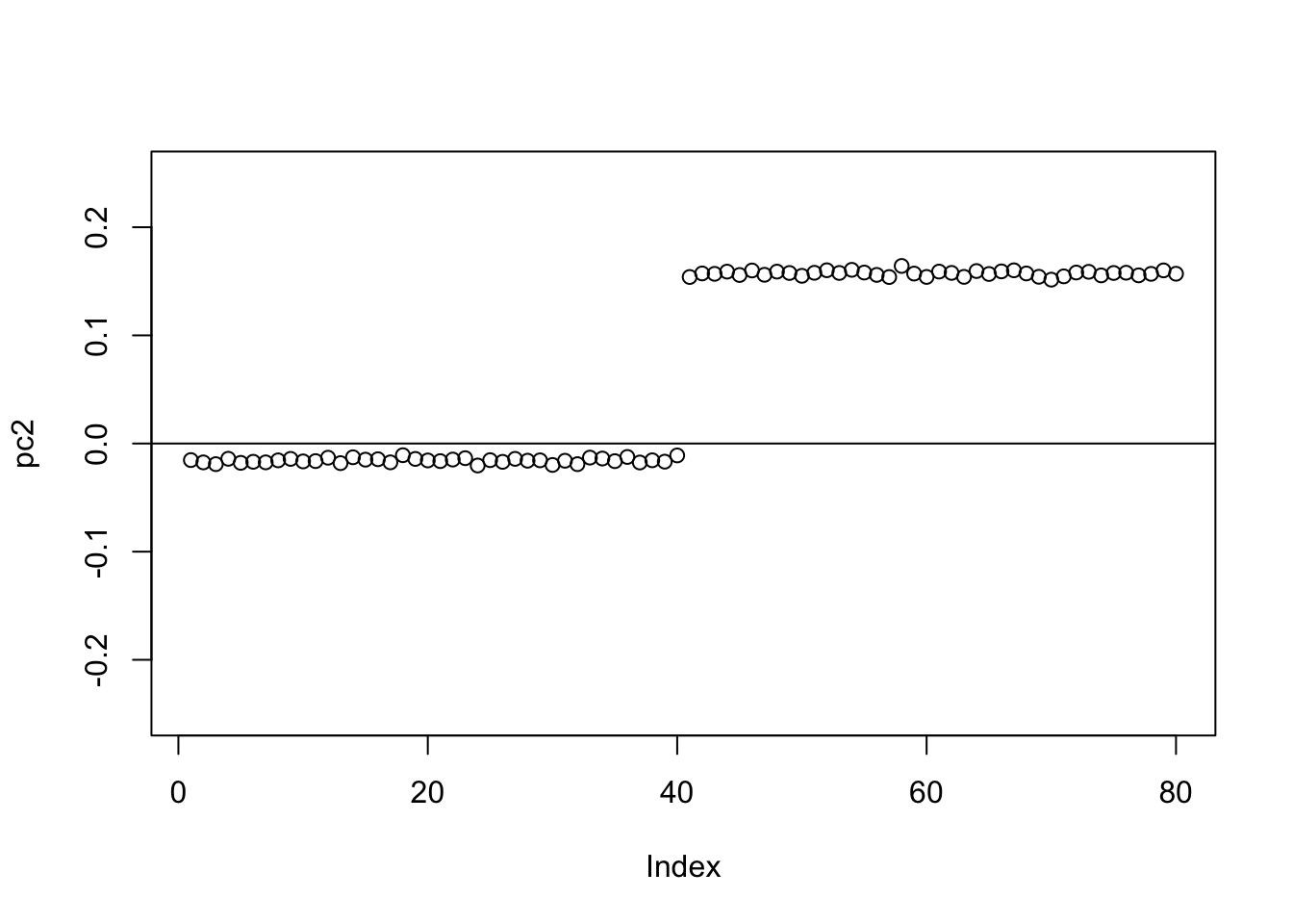
If one uses a completely random initialization then the eb method will often (but not always) zero things out completely on the first iteration:
set.seed(1)
v = cbind(rnorm(2*n))
v= v/sqrt(sum(v^2))
sigma = sqrt(mean(S^2))
v = eb_power_update_r1(S,v,ebnm_point_laplace,sigma)
plot(v,ylim=c(-0.25,0.25))
abline(h=0)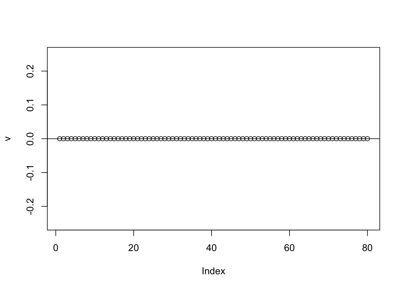
We can help avoid this here by doing a single iteration of the power method before moving to EB (because the matrix is very low rank the single iteration moves us quickly to the right subspace). Here the point-laplace gives a 0-1 split of the top 2 branches.
set.seed(1)
v = cbind(rnorm(2*n))
v= v/sqrt(sum(v^2))
sigma = sqrt(mean(S^2))

v = power_update_r1(S,v)
plot(v,ylim=c(-0.25,0.25))
for(i in 1:100){
  v = eb_power_update_r1(S,v,ebnm_point_laplace,sigma)
}
plot(v,ylim=c(-0.25,0.25))
abline(h=0)
The point exponential performs similarly, but the “0” part is slightly non-zero. This is possibly due to the posterior mean reflecting a small probability of coming from the exponential part. (This is not a convergence issue - it remains with more iterations, not shown.)
set.seed(1)
v = cbind(rnorm(2*n))
v= v/sqrt(sum(v^2))
sigma = sqrt(mean(S^2))

v = power_update_r1(S,v)
plot(v,ylim=c(-0.25,0.25))
for(i in 1:100){
  v = eb_power_update_r1(S,v,ebnm_point_exponential,sigma)
}
plot(v,ylim=c(-0.25,0.25))
abline(h=0)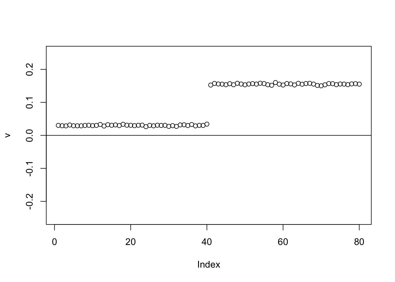
Try further running binormal - it moves things to 0.
for(i in 1:100){
  v = eb_power_update_r1(S,v,ebnm_binormal,sigma)
}
plot(v, ylim=c(-0.25,0.25))
abline(h=0)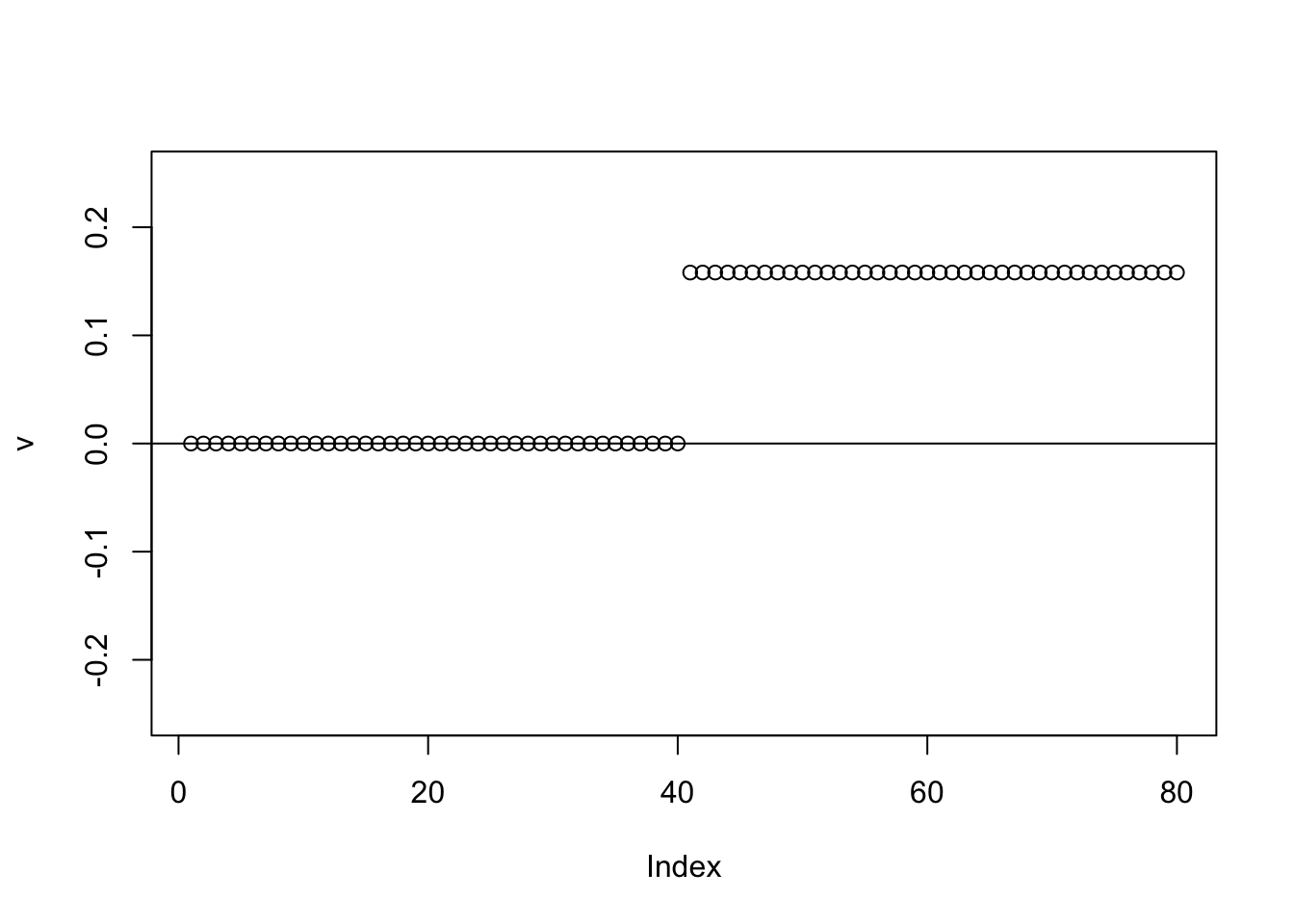
Here running binormal from a random starting point gives the constant vector. (Not a bad solution in principle, but not what we are looking for)
set.seed(1)
v = cbind(rnorm(2*n))
v= v/sqrt(sum(v^2))
sigma = sqrt(mean(S^2))

v = power_update_r1(S,v)
plot(v,ylim=c(-0.25,0.25))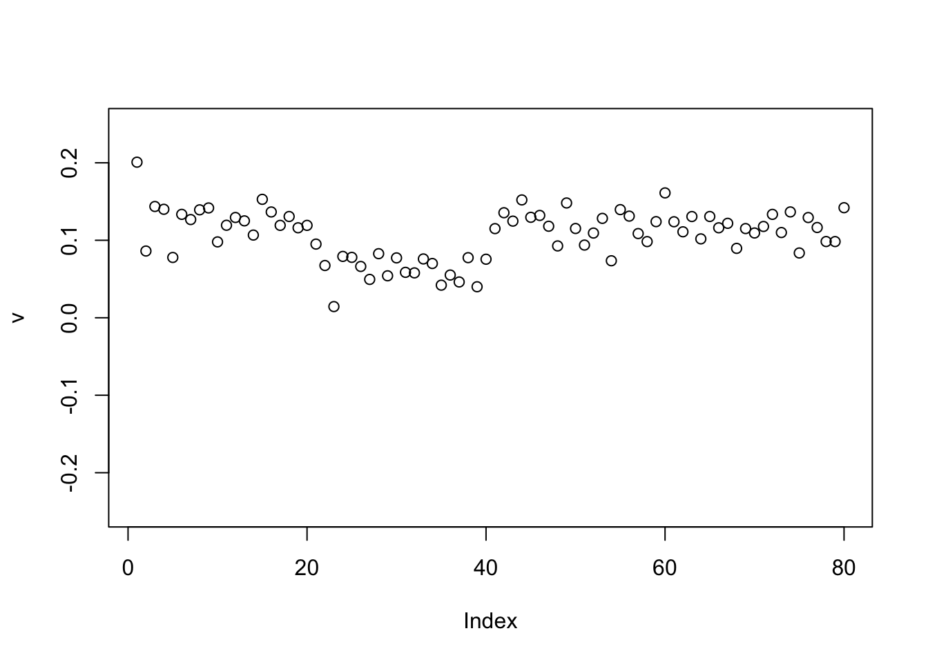
for(i in 1:100){
  v = eb_power_update_r1(S,v,ebnm_binormal,sigma)
}
plot(v,ylim=c(-0.25,0.25))
abline(h=0)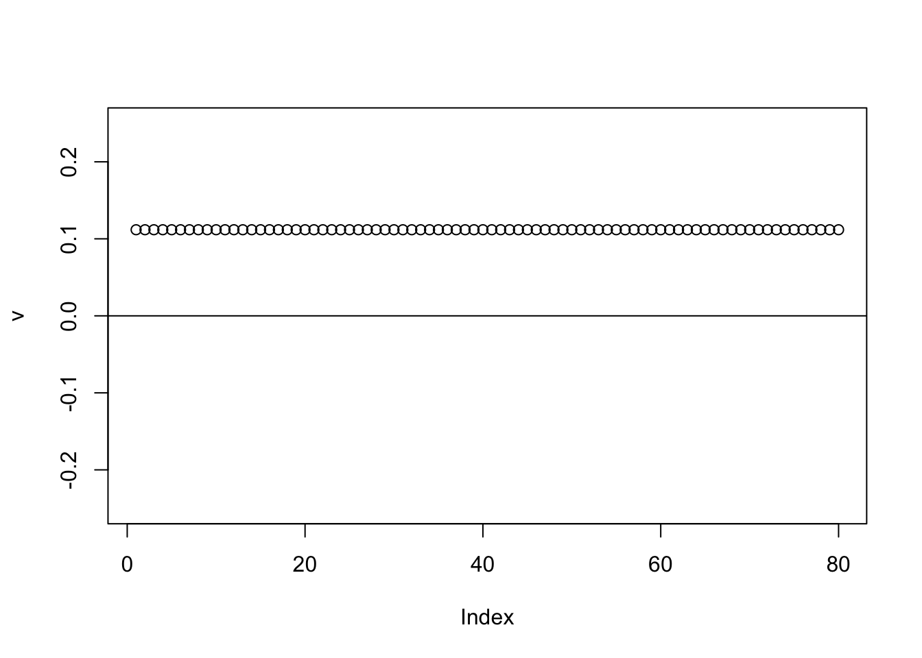
Tree model - stronger diagonal
To try to make things interesting I make the diagonal stronger, so that there is ambiguity about whether to split on the top branch or the population-specific branches. I’m hoping to create a situation where the point exponential gives us a non tree-like solution that captures no single branch (ie captures multiple branches).
set.seed(1)
S = x %*% diag(c(1,1,8,8,8,8)) %*% t(x) + E
image(S)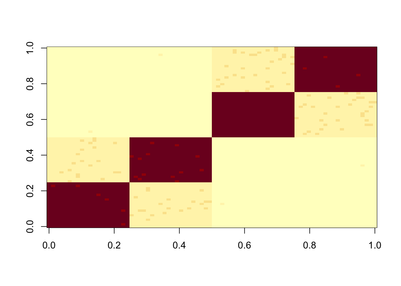
Check the PCs. They don’t change much from the original symmetric case.
S.svd = svd(S)
S.svd$d[1:10]
[1] 199.947650 199.868321 160.210573 159.963782 2.440134 2.398514
[7] 2.311234 2.231927 2.182422 2.154607pc1 = cbind(S.svd$v[,1])
pc2 = cbind(S.svd$v[,2])
plot(pc1,ylim=c(-0.25,0.25))
abline(h=0)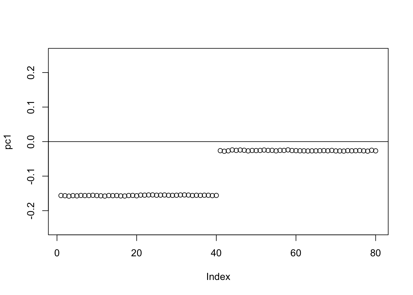
plot(pc2,ylim=c(-0.25,0.25))
abline(h=0)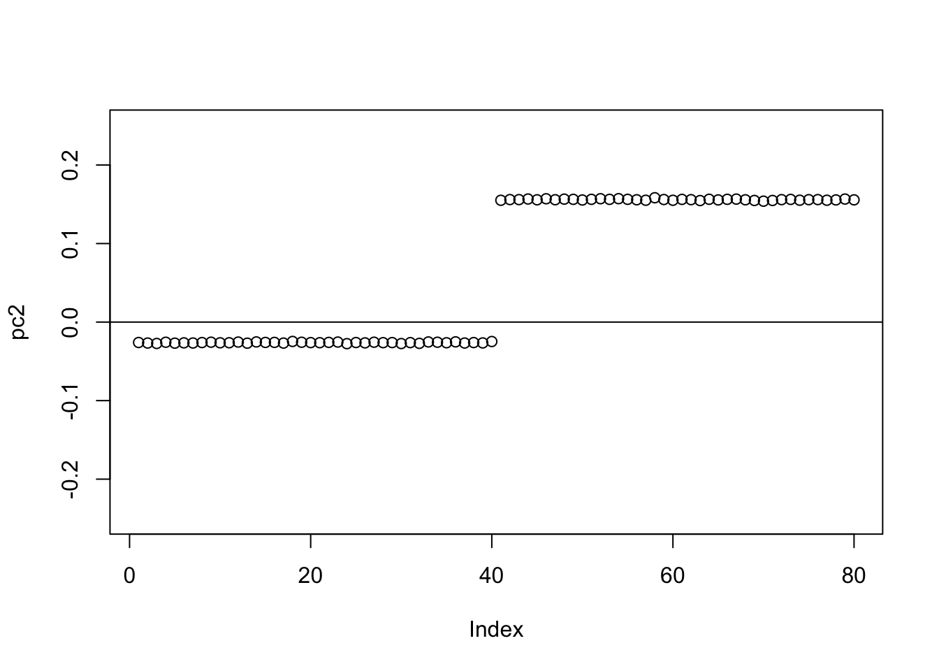
Again, point-laplace gives a 0-1 split of the top 2 branches (even though initialized here from something closer to a split of 3 populations vs 1)
set.seed(1)
v = cbind(rnorm(2*n))
v= v/sqrt(sum(v^2))
sigma = sqrt(mean(S^2))

v = power_update_r1(S,v)
plot(v,ylim=c(-0.25,0.25))
for(i in 1:100){
  v = eb_power_update_r1(S,v,ebnm_point_laplace,sigma)
}
plot(v,ylim=c(-0.25,0.25))
abline(h=0)
The point exponential performs similarly, but the “0” part again slightly non-zero.
set.seed(1)
v = cbind(rnorm(2*n))
v= v/sqrt(sum(v^2))
sigma = sqrt(mean(S^2))

v = power_update_r1(S,v)
plot(v,ylim=c(-0.25,0.25))
for(i in 1:100){
  v = eb_power_update_r1(S,v,ebnm_point_exponential,sigma)
}
plot(v,ylim=c(-0.25,0.25))
abline(h=0)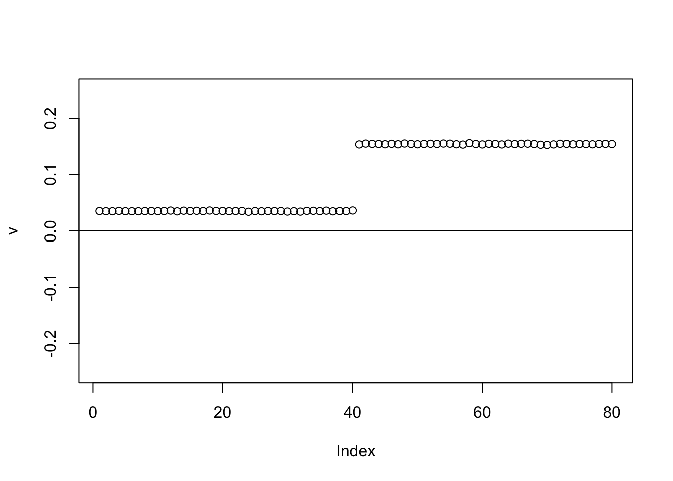
This time we use generalized binary, which like the binormal moves that non-zero element to 0.
for(i in 1:100){
  v = eb_power_update_r1(S,v,ebnm_generalized_binary,sigma)
}
plot(v, ylim=c(-0.25,0.25))
abline(h=0)
Here running binormal from a random starting point gives a 3-population split. It is another illustration of why running binormal from a random starting point may not be a good idea.
set.seed(1)
v = cbind(rnorm(2*n))
v= v/sqrt(sum(v^2))
sigma = sqrt(mean(S^2))

v = power_update_r1(S,v)
plot(v,ylim=c(-0.25,0.25))
for(i in 1:100){
  v = eb_power_update_r1(S,v,ebnm_binormal,sigma)
}
plot(v,ylim=c(-0.25,0.25))
abline(h=0)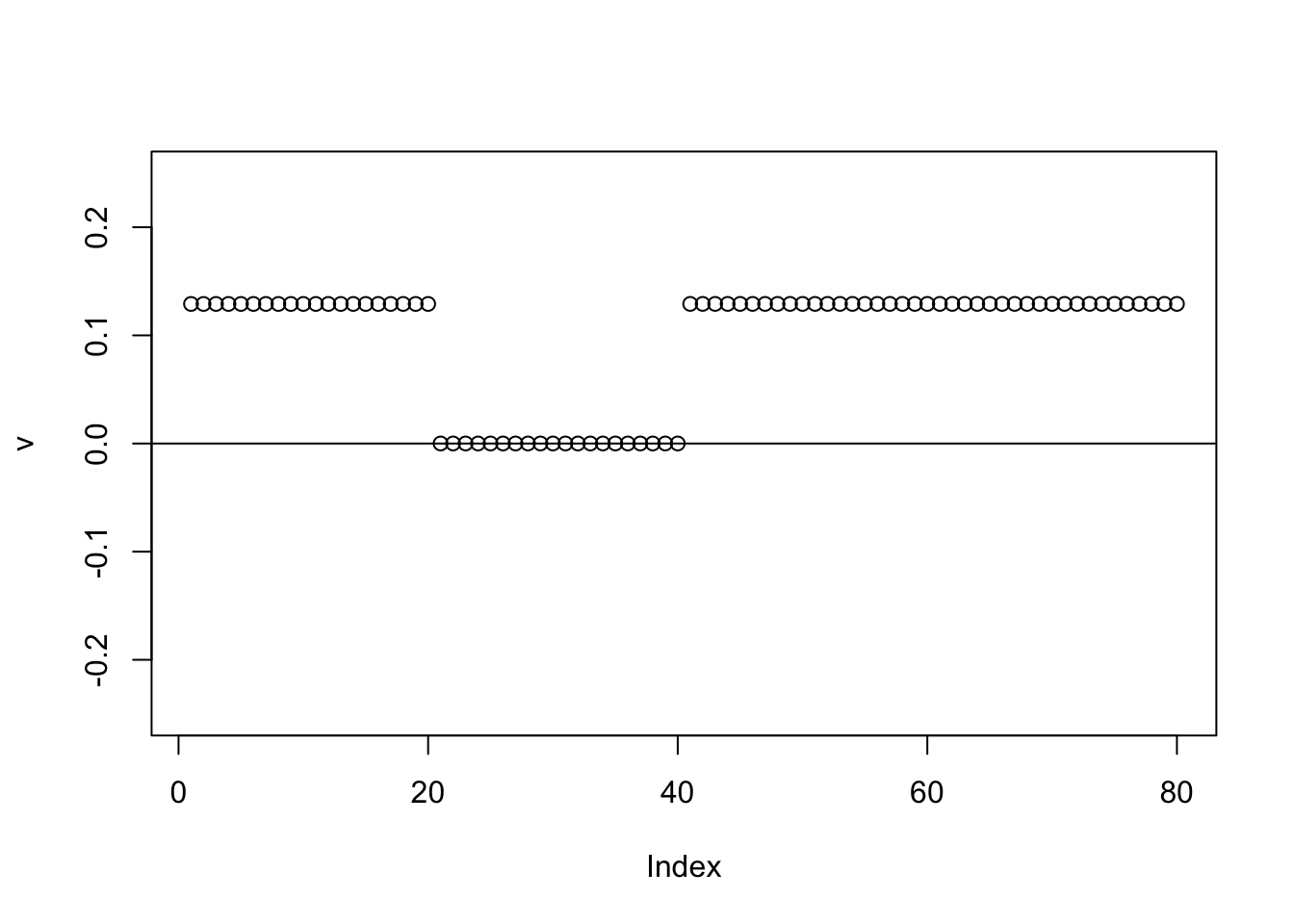
The same happens for the GB prior:
set.seed(1)
v = cbind(rnorm(2*n))
v= v/sqrt(sum(v^2))
sigma = sqrt(mean(S^2))

v = power_update_r1(S,v)
plot(v,ylim=c(-0.25,0.25))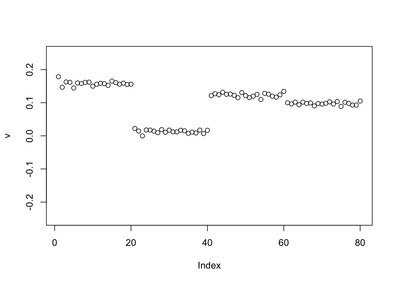
for(i in 1:100){
  v = eb_power_update_r1(S,v,ebnm_generalized_binary,sigma)
}
plot(v,ylim=c(-0.25,0.25))
abline(h=0)
Tree model - centered
Now we try centering the tree.
set.seed(1)
S = x %*% diag(c(1,1,1,1,1,1)) %*% t(x) + E
S = S-mean(S)
image(S)
Check the PCs. The top 2 PCs have similar eigenvalues. The first one splits the top two branches; the second one also splits them, but is almost constant.
S.svd = svd(S)
S.svd$d[1:10]
[1] 59.917919 20.283599 20.025645 2.447187 2.404583 2.313047 2.263498
[8] 2.199084 2.160395 2.091650pc1 = cbind(S.svd$v[,1])
pc2 = cbind(S.svd$v[,2])
plot(pc1,ylim=c(-0.25,0.25))
abline(h=0)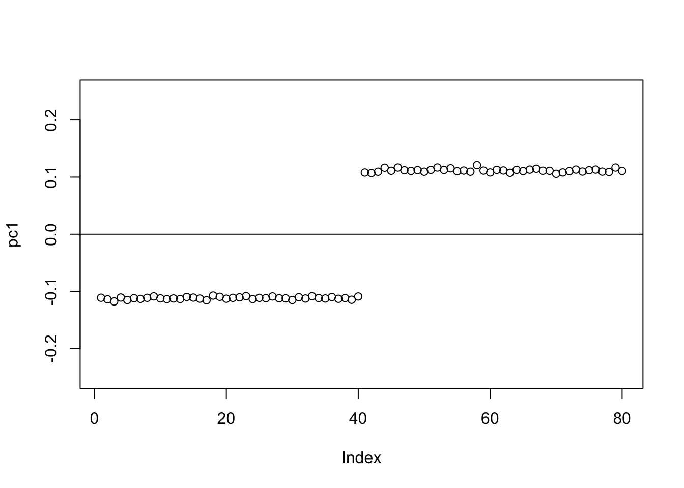
plot(pc2,ylim=c(-0.25,0.25))
abline(h=0)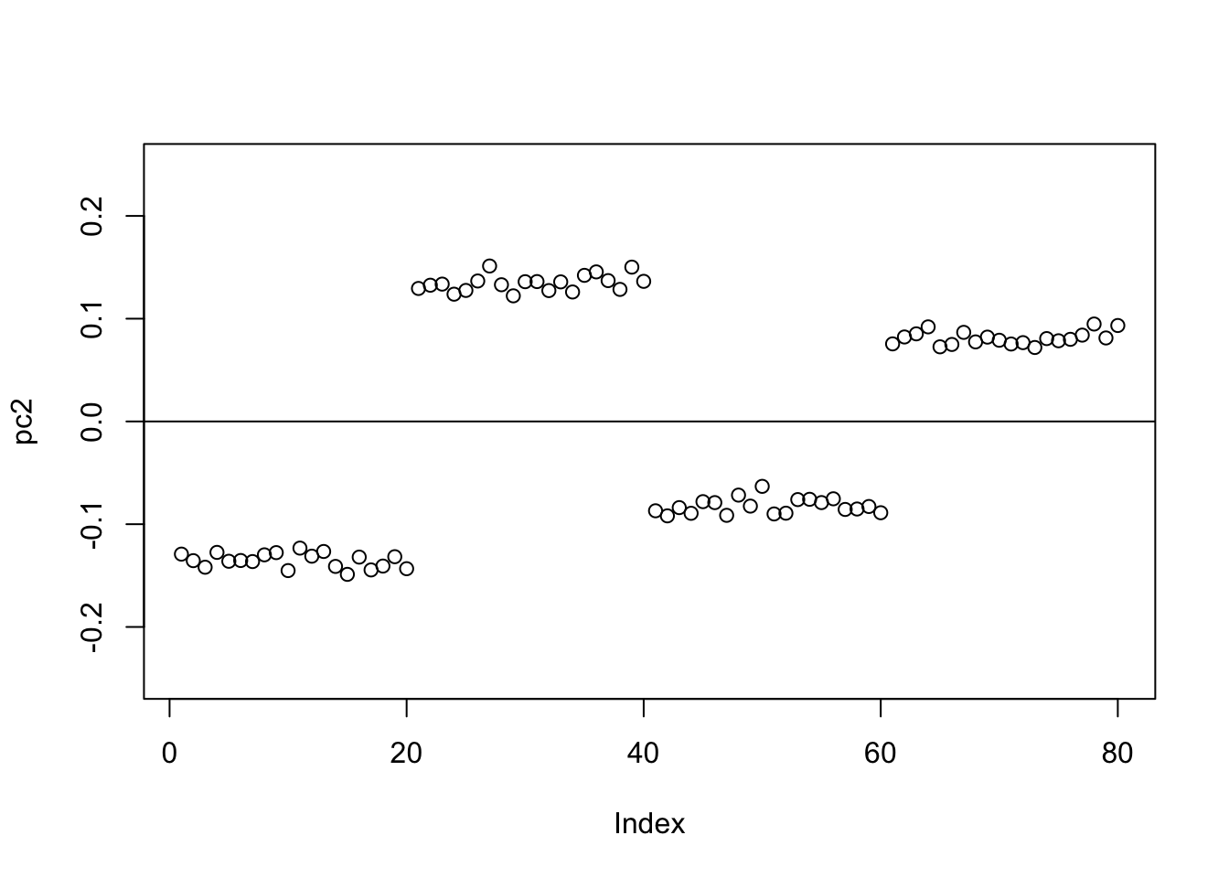
Now the point-laplace gives a +-1 split of the top 2 branches.
set.seed(1)
v = cbind(rnorm(2*n))
v= v/sqrt(sum(v^2))
sigma = sqrt(mean(S^2))

v = power_update_r1(S,v)
plot(v,ylim=c(-0.25,0.25))
for(i in 1:100){
  v = eb_power_update_r1(S,v,ebnm_point_laplace,sigma)
}
plot(v,ylim=c(-0.25,0.25))
abline(h=0)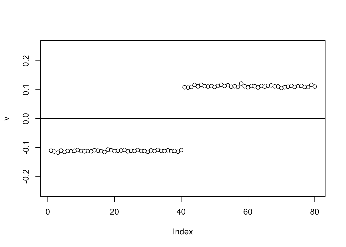
The point exponential produces a 0-1 split.
set.seed(1)
v = cbind(rnorm(2*n))
v= v/sqrt(sum(v^2))
sigma = sqrt(mean(S^2))

v = power_update_r1(S,v)
plot(v,ylim=c(-0.25,0.25))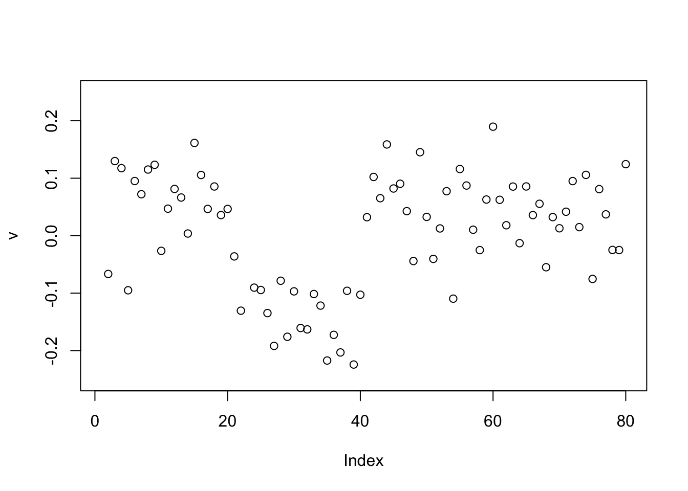
for(i in 1:100){
  v = eb_power_update_r1(S,v,ebnm_point_exponential,sigma)
}
plot(v,ylim=c(-0.25,0.25))
abline(h=0)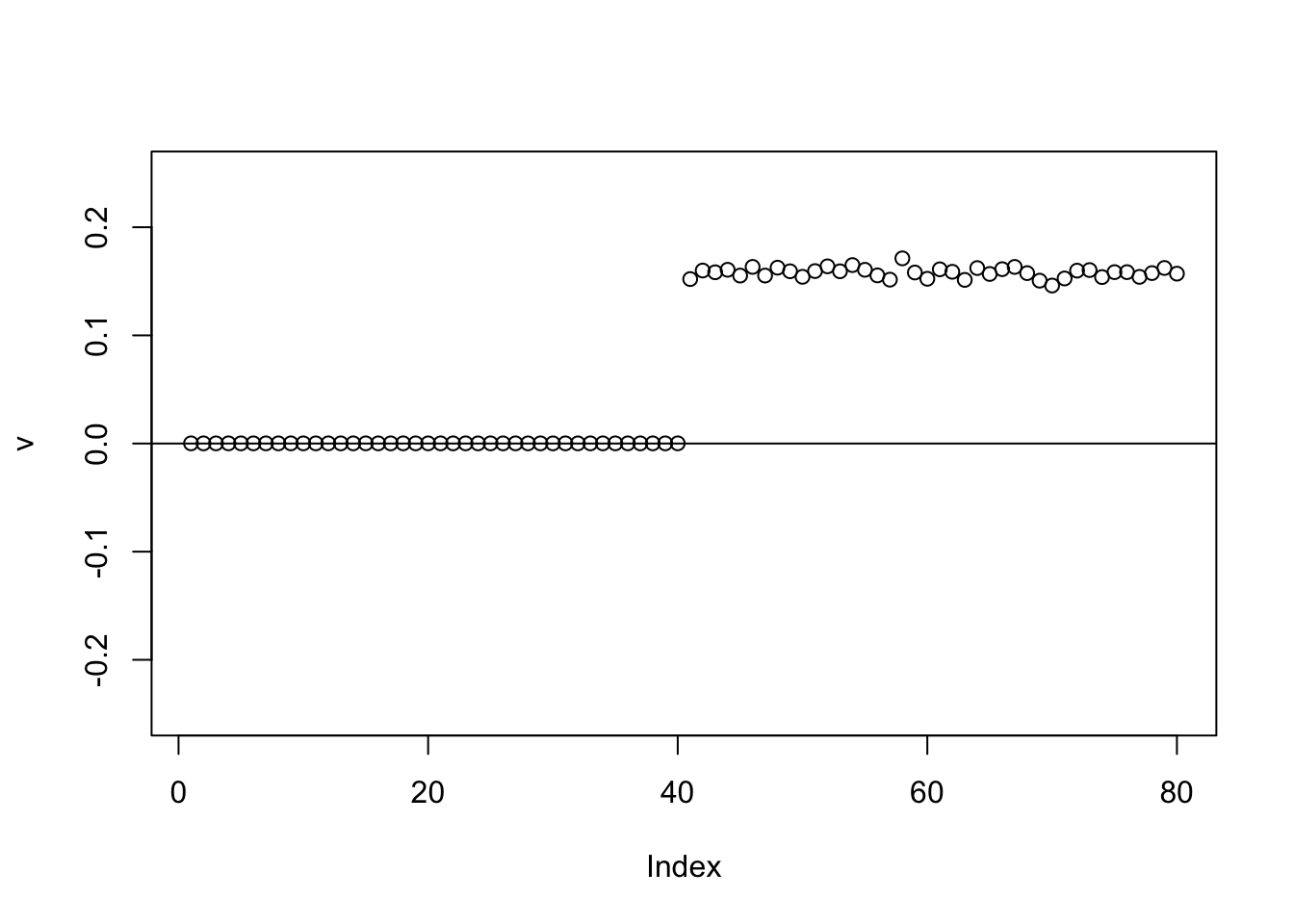
Here running binormal from a random starting point also gives the 0-1 split.
set.seed(1)
v = cbind(rnorm(2*n))
v= v/sqrt(sum(v^2))
sigma = sqrt(mean(S^2))

v = power_update_r1(S,v)
plot(v,ylim=c(-0.25,0.25))
for(i in 1:100){
  v = eb_power_update_r1(S,v,ebnm_binormal,sigma)
}
plot(v,ylim=c(-0.25,0.25))
abline(h=0)
Rank K
# model is  S \sim VDV' + E with eb prior on V
eb_power_update = function(S,v,d,ebnm_fn){
  K = ncol(v)
  sigma2=mean((S-v %*% diag(d,nrow=length(d)) %*% t(v))^2)

  for(k in 1:K){
    U = v[,-k,drop=FALSE]
    D = diag(d[-k],nrow=length(d[-k]))

    newv = (S %*% v[,k,drop=FALSE] - U %*% D %*% t(U) %*% v[,k,drop=FALSE] )
    if(!all(newv==0)){
      fit.ebnm = ebnm_fn(newv,sqrt(sigma2))
      newv = fit.ebnm$posterior$mean
      if(!all(newv==0)){
        newv = newv/sqrt(sum(newv^2 + fit.ebnm$posterior$sd^2))
      }
    }
    v[,k] = newv
    d[k] = t(v[,k]) %*% S %*% v[,k] - t(v[,k]) %*% U %*% D %*% t(U) %*% v[,k]
  }
  return(list(v=v,d=d))
}

#helper function
compute_sqerr = function(S,fit){
  sum((S-fit$v %*% diag(fit$d,nrow=length(fit$d)) %*% t(fit$v))^2)
}

# a random initialization
random_init = function(S,K,nonneg = FALSE){
  n = nrow(S)
  v = matrix(nrow=n,ncol=K)

  for(k in 1:K){
    v[,k] = cbind(rnorm(n)) # initialize v
    if(nonneg)
        v[,k] = pmax(v[,k],0)
    v[,k] = v[,k]/sum(v[,k]^2)
  }
  d = rep(1e-8,K)
  return(list(v=v,d=d))
}
Tree structured data
Simulate data under a tree model (with very small errors)
set.seed(1)
n = 40
x = cbind(c(rep(1,n),rep(0,n)), c(rep(0,n),rep(1,n)), c(rep(1,n/2),rep(0,3*n/2)), c(rep(0,n/2), rep(1,n/2), rep(0,n)), c(rep(0,n),rep(1,n/2),rep(0,n/2)), c(rep(0,3*n/2),rep(1,n/2)))
E = matrix(0.01*rexp(2*n*2*n),nrow=2*n)
E = E+t(E) #symmetric errors
S = x %*% diag(c(1,1,1,1,1,1)) %*% t(x) + E
image(S)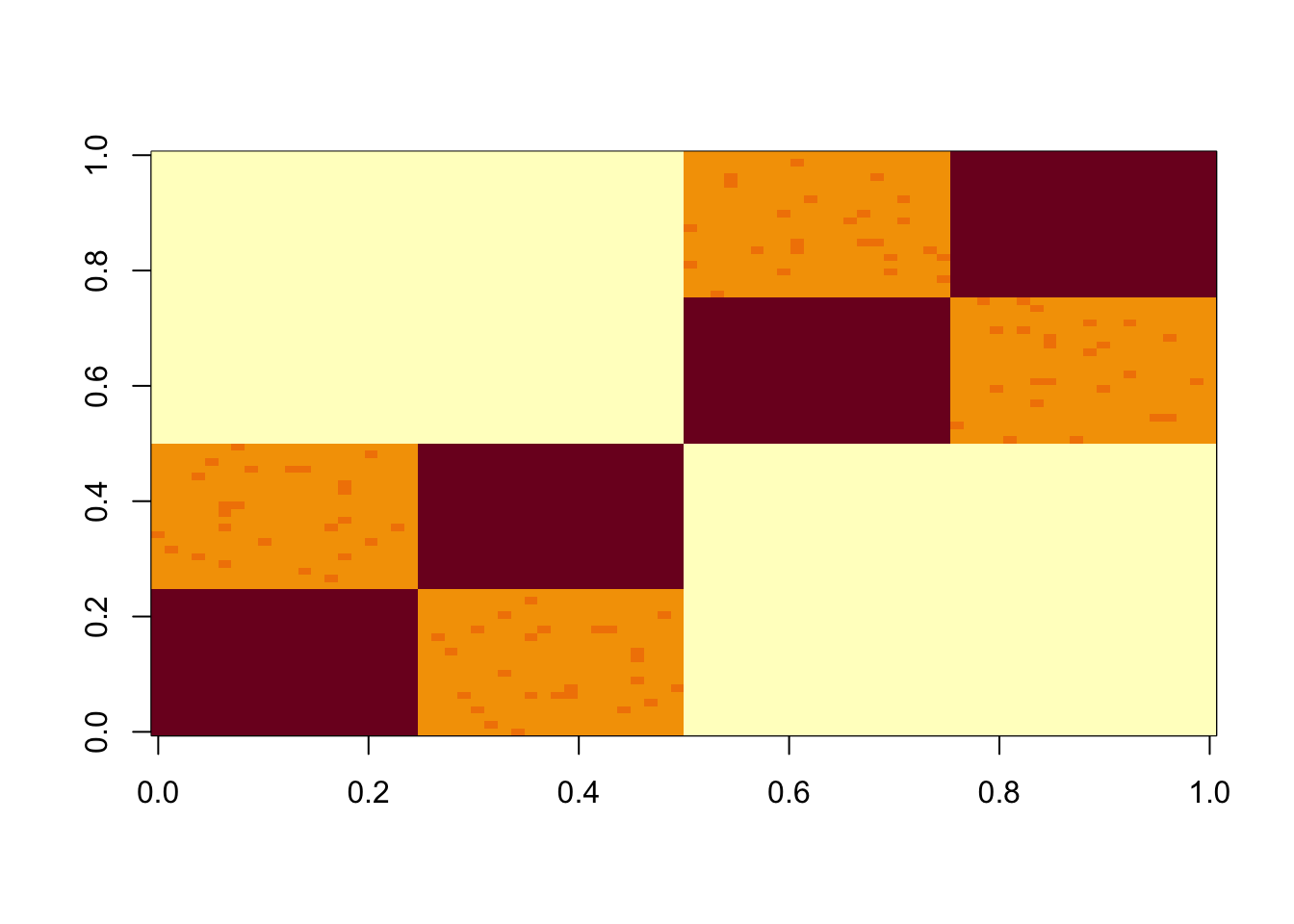
Run multiple factors
Here I run with \(K=9\) and point-exponential. It finds a rank 4 solution, essentially zeroing out the other 5. One can compare this with non-negative without the EB approach here.
set.seed(2)
fit = random_init(S,9,nonneg=TRUE)
err = rep(0,10)
err[1] = sum((S-fit$v %*% diag(fit$d) %*% t(fit$v))^2)
for(i in 2:100){
  fit = eb_power_update(S,fit$v,fit$d,ebnm_point_exponential)
  err[i] = sum((S-fit$v %*% diag(fit$d) %*% t(fit$v))^2)
}
plot(err)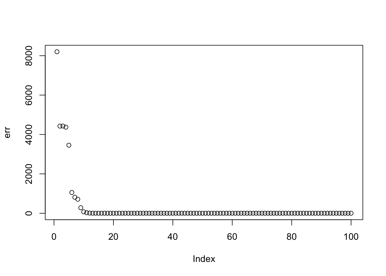
par(mfcol=c(3,3),mai=rep(0.3,4))
for(i in 1:9){plot(fit$v[,i],main=paste0(trunc(fit$d[i])))}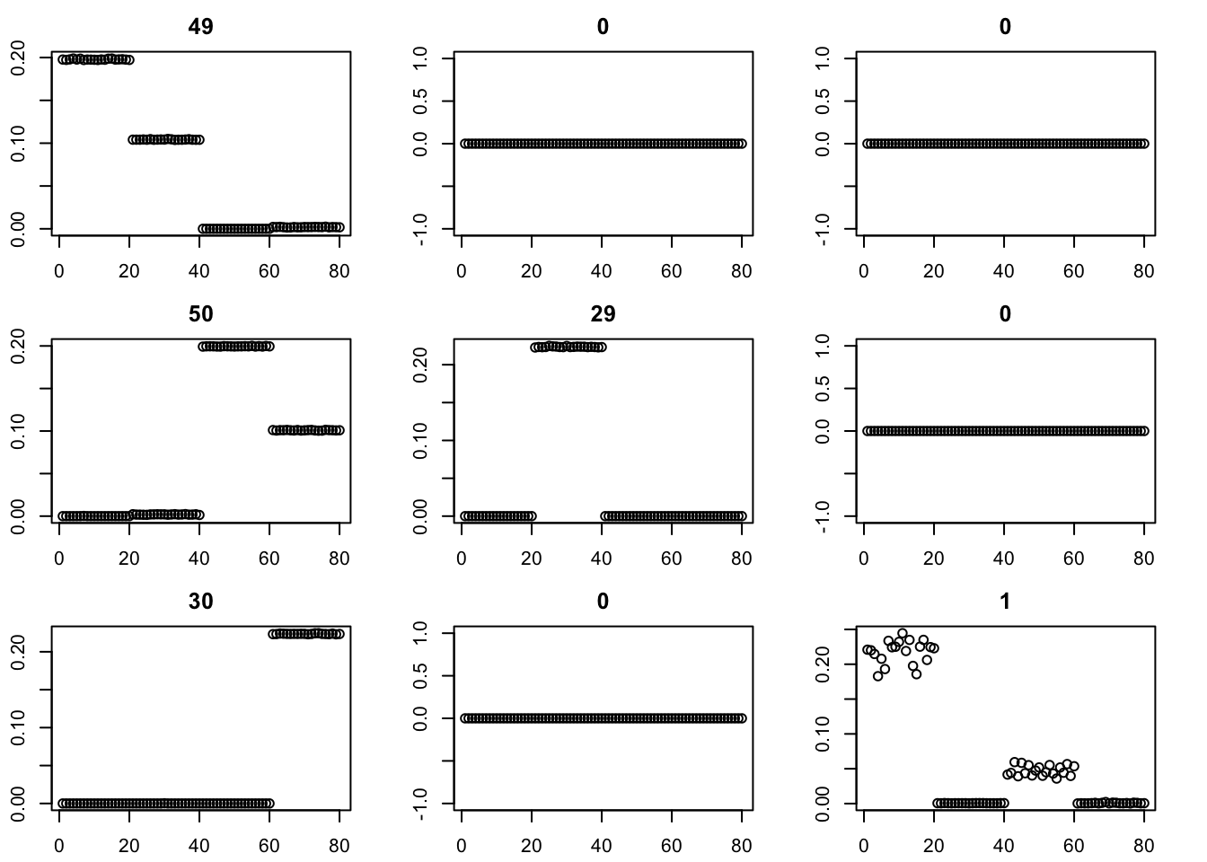
Here I try the generalized binary prior. So far I’m finding this does not work well, especially if started from random starting point. I debugged and found that what happens is that generally the v are bounded away from 0. So the gb prior puts all its weight on the non-null normal component and does not shrink anything. (Is it worth using a laplace for the non-null component?) The point exponential does not have that problem - it shrinks the smallest values towards 0, and eventually gets to a point where everything is 0. It seems clear that using the gb prior from random initialization is not going to work.
set.seed(2)
fit = random_init(S,9, nonneg=TRUE)
err = rep(0,10)
err[1] = sum((S-fit$v %*% diag(fit$d) %*% t(fit$v))^2)

for(i in 2:10){
  fit = eb_power_update(S,fit$v,fit$d,ebnm_generalized_binary)
  err[i] = sum((S-fit$v %*% diag(fit$d) %*% t(fit$v))^2)
}
plot(err)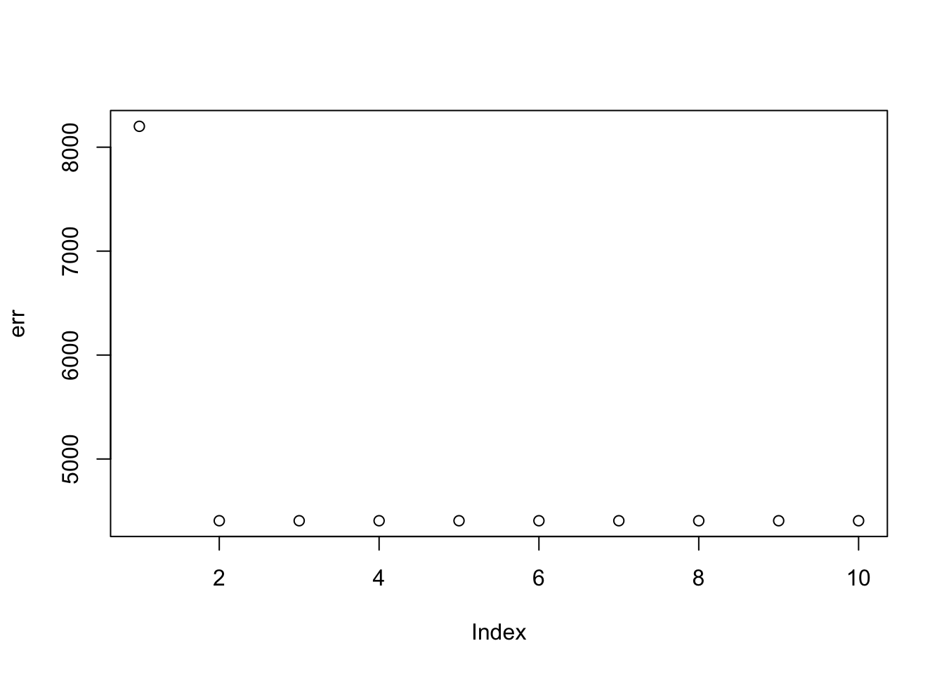
par(mfcol=c(3,3),mai=rep(0.3,4))
for(i in 1:9){plot(fit$v[,i],main=paste0(trunc(fit$d[i])))}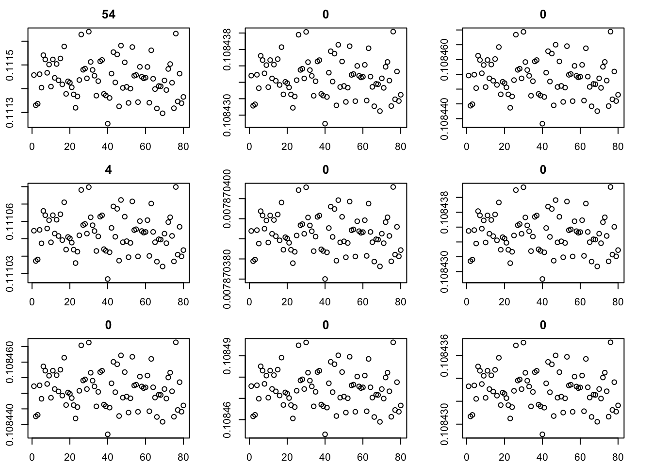
Here we try initializing GB with point-exponential. It only changes the fit very little.
set.seed(2)
fit = random_init(S,9,nonneg=TRUE)

for(i in 1:100){
  fit = eb_power_update(S,fit$v,fit$d,ebnm_point_exponential)
}
par(mfcol=c(3,3),mai=rep(0.3,4))
for(i in 1:9){plot(fit$v[,i],main=paste0(trunc(fit$d[i])))}
for(i in 1:100){
  fit = eb_power_update(S,fit$v,fit$d,ebnm_generalized_binary)
}
par(mfcol=c(3,3),mai=rep(0.3,4))
for(i in 1:9){plot(fit$v[,i],main=paste0(trunc(fit$d[i])))}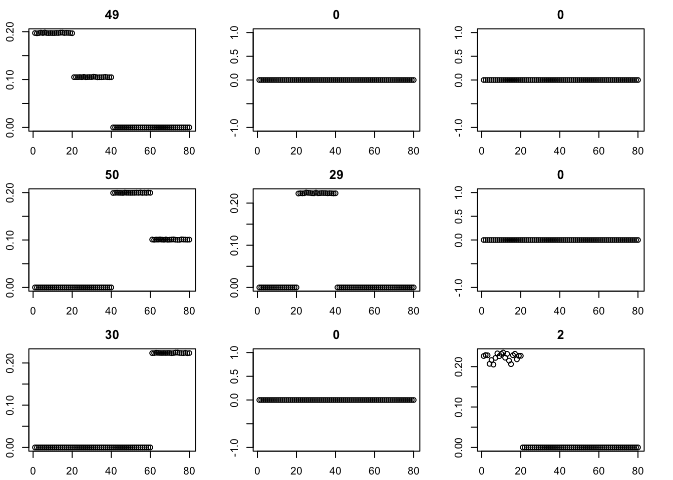
The binormal prior provides a more bimodal solution. (Note: although not seen here, I have seen issues with it including a factor that puts two non-neighboring populations together.)
for(i in 1:100){
  fit = eb_power_update(S,fit$v,fit$d,ebnm_binormal)
  err[i] = compute_sqerr(S,fit)
}
par(mfcol=c(3,3),mai=rep(0.3,4))
for(i in 1:9){plot(fit$v[,i],main=paste0(trunc(fit$d[i])))}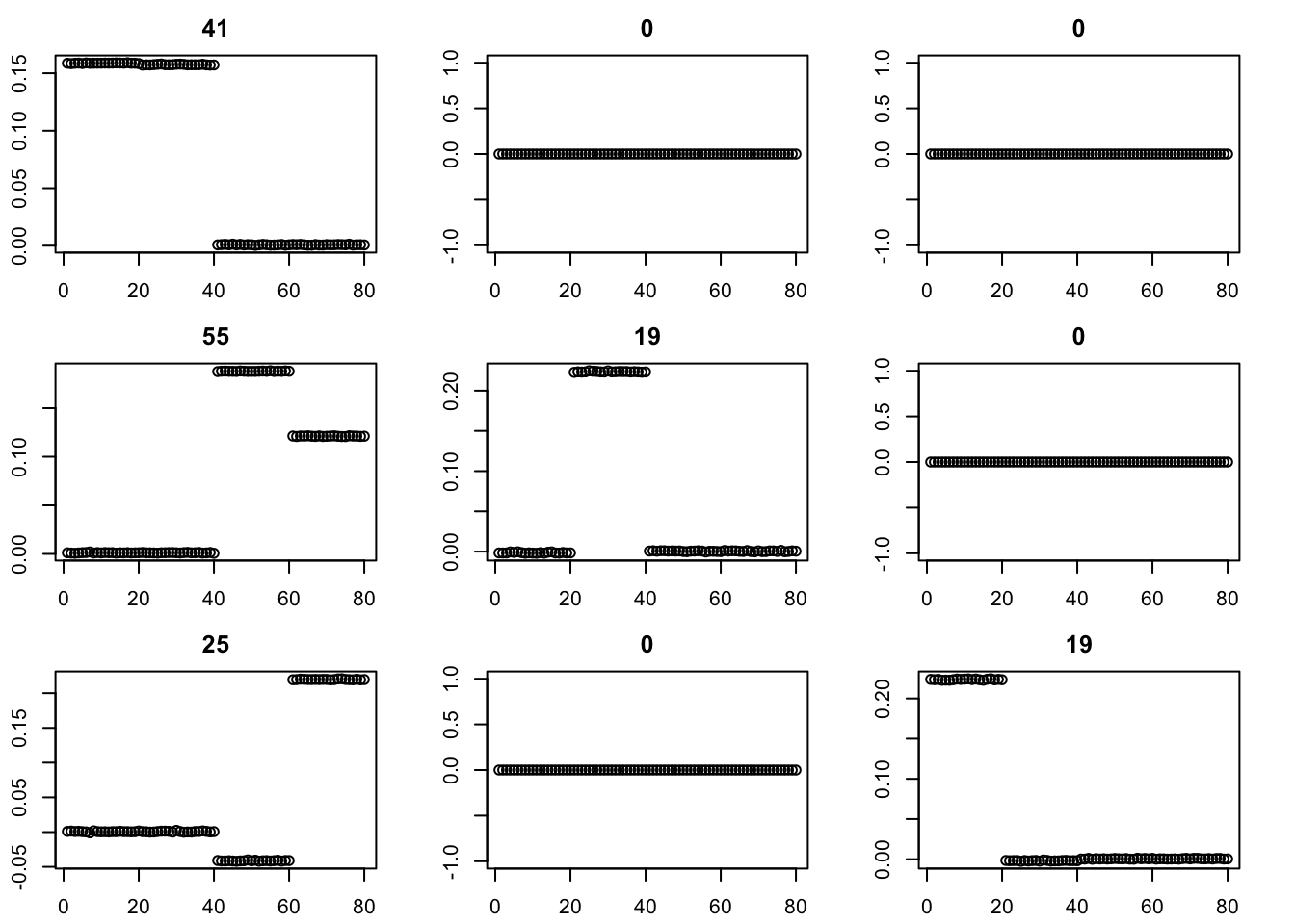
for(i in 1:100){
  fit = eb_power_update(S,fit$v,fit$d,ebnm_binormal)
}
par(mfcol=c(3,3),mai=rep(0.3,4))
for(i in 1:9){plot(fit$v[,i],main=paste0(trunc(fit$d[i])))}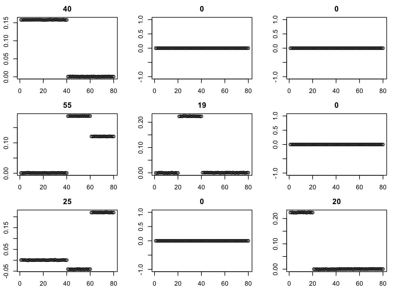
SVD initialization
I’m going to try initializing with SVD, then running point-laplace, then running GB, similar to the strategy in the GBCD paper. (Note: here I initialize with the svd values for d; an alternative is to set these to be very small and just use the v from svd to initialize.)
set.seed(2)
S.svd = svd(S)

fit = list(v=S.svd$u[,1:4],d=S.svd$d[1:4]) #rep(1e-8,4)) #init d to be very small

err = rep(0,10)
err[1] = compute_sqerr(S,fit)

for(i in 2:100){
  fit = eb_power_update(S,fit$v,fit$d,ebnm_point_laplace)
  err[i] = compute_sqerr(S,fit)
}
par(mfcol=c(3,3),mai=rep(0.3,4))
for(i in 1:4){plot(fit$v[,i],main=paste0(trunc(fit$d[i])))}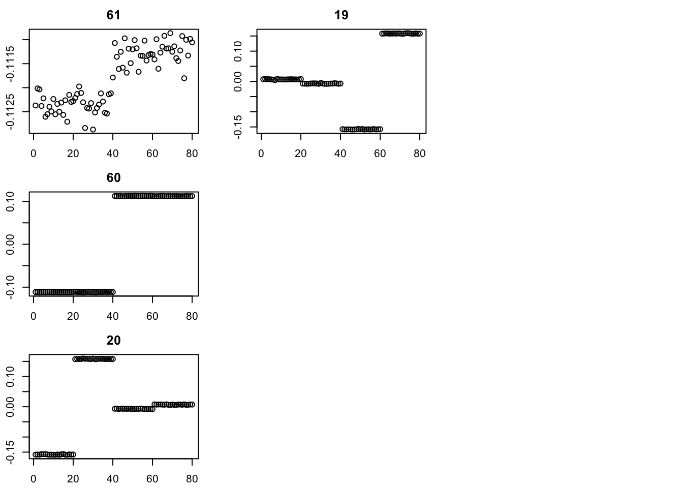
split_v = function(v){
  v = cbind(pmax(v,0),pmax(-v,0))
}

fit$v = split_v(fit$v)
fit$d= rep(fit$d/2,2)

for(i in 2:100){
  fit = eb_power_update(S,fit$v,fit$d,ebnm_point_exponential)
  err[i] = compute_sqerr(S,fit)
}
par(mfcol=c(3,3),mai=rep(0.3,4))
for(i in 1:8){plot(fit$v[,i],main=paste0(trunc(fit$d[i])))}
fit.pe = fit # save for later use

for(i in 2:200){
  fit = eb_power_update(S,fit$v,fit$d,ebnm_generalized_binary)
  err[i] = compute_sqerr(S,fit)
}
par(mfcol=c(3,3),mai=rep(0.3,4))
for(i in 1:8){plot(fit$v[,i],main=paste0(trunc(fit$d[i])))}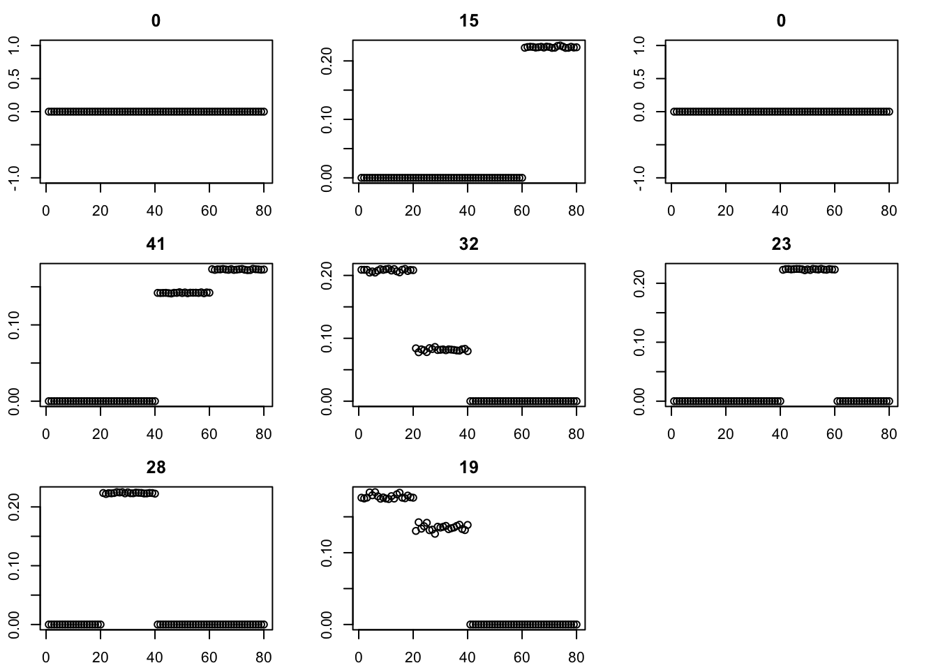
Try binormal instead, initialized from point-exp. This works better.
fit = fit.pe
for(i in 2:200){
  fit = eb_power_update(S,fit$v,fit$d,ebnm_binormal)
  err[i] = compute_sqerr(S,fit)
}
par(mfcol=c(3,3),mai=rep(0.3,4))
for(i in 1:8){plot(fit$v[,i],main=paste0(trunc(fit$d[i])))}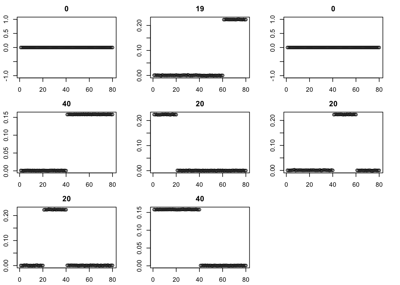
sessionInfo()R version 4.4.2 (2024-10-31)
Platform: aarch64-apple-darwin20
Running under: macOS Sequoia 15.3.1
Matrix products: default
BLAS: /Library/Frameworks/R.framework/Versions/4.4-arm64/Resources/lib/libRblas.0.dylib
LAPACK: /Library/Frameworks/R.framework/Versions/4.4-arm64/Resources/lib/libRlapack.dylib; LAPACK version 3.12.0
locale:
[1] en_US.UTF-8/en_US.UTF-8/en_US.UTF-8/C/en_US.UTF-8/en_US.UTF-8
time zone: America/Chicago
tzcode source: internal
attached base packages:
[1] stats graphics grDevices utils datasets methods base
other attached packages:
[1] ebnm_1.1-2
loaded via a namespace (and not attached):
[1] sass_0.4.9 generics_0.1.3 ashr_2.2-63 stringi_1.8.4
[5] lattice_0.22-6 digest_0.6.37 magrittr_2.0.3 evaluate_1.0.3
[9] grid_4.4.2 fastmap_1.2.0 rprojroot_2.0.4 workflowr_1.7.1
[13] jsonlite_1.8.9 Matrix_1.7-2 whisker_0.4.1 mixsqp_0.3-54
[17] promises_1.3.2 scales_1.3.0 truncnorm_1.0-9 invgamma_1.1
[21] jquerylib_0.1.4 cli_3.6.3 rlang_1.1.5 deconvolveR_1.2-1
[25] munsell_0.5.1 splines_4.4.2 cachem_1.1.0 yaml_2.3.10
[29] tools_4.4.2 SQUAREM_2021.1 dplyr_1.1.4 colorspace_2.1-1
[33] ggplot2_3.5.1 httpuv_1.6.15 vctrs_0.6.5 R6_2.5.1
[37] lifecycle_1.0.4 git2r_0.35.0 stringr_1.5.1 fs_1.6.5
[41] trust_0.1-8 irlba_2.3.5.1 pkgconfig_2.0.3 pillar_1.10.1
[45] bslib_0.9.0 later_1.4.1 gtable_0.3.6 glue_1.8.0
[49] Rcpp_1.0.14 xfun_0.50 tibble_3.2.1 tidyselect_1.2.1
[53] rstudioapi_0.17.1 knitr_1.49 htmltools_0.5.8.1 rmarkdown_2.29
[57] compiler_4.4.2 horseshoe_0.2.0