fit Lasso by EM
Matthew Stephens
2020-06-02
Last updated: 2020-06-18
Checks: 7 0
Knit directory: misc/analysis/
This reproducible R Markdown analysis was created with workflowr (version 1.6.1). The Checks tab describes the reproducibility checks that were applied when the results were created. The Past versions tab lists the development history.
Great! Since the R Markdown file has been committed to the Git repository, you know the exact version of the code that produced these results.
Great job! The global environment was empty. Objects defined in the global environment can affect the analysis in your R Markdown file in unknown ways. For reproduciblity it’s best to always run the code in an empty environment.
The command set.seed(1) was run prior to running the code in the R Markdown file. Setting a seed ensures that any results that rely on randomness, e.g. subsampling or permutations, are reproducible.
Great job! Recording the operating system, R version, and package versions is critical for reproducibility.
Nice! There were no cached chunks for this analysis, so you can be confident that you successfully produced the results during this run.
Great job! Using relative paths to the files within your workflowr project makes it easier to run your code on other machines.
Great! You are using Git for version control. Tracking code development and connecting the code version to the results is critical for reproducibility.
The results in this page were generated with repository version 51b89bb. See the Past versions tab to see a history of the changes made to the R Markdown and HTML files.
Note that you need to be careful to ensure that all relevant files for the analysis have been committed to Git prior to generating the results (you can use wflow_publish or wflow_git_commit). workflowr only checks the R Markdown file, but you know if there are other scripts or data files that it depends on. Below is the status of the Git repository when the results were generated:
Ignored files:
    Ignored:    .DS_Store
    Ignored:    .Rhistory
    Ignored:    .Rproj.user/
    Ignored:    analysis/.RData
    Ignored:    analysis/.Rhistory
    Ignored:    analysis/ALStruct_cache/
    Ignored:    data/.Rhistory
    Ignored:    data/pbmc/

Untracked files:
    Untracked:  .dropbox
    Untracked:  Icon
    Untracked:  analysis/GHstan.Rmd
    Untracked:  analysis/GTEX-cogaps.Rmd
    Untracked:  analysis/PACS.Rmd
    Untracked:  analysis/Rplot.png
    Untracked:  analysis/SPCAvRP.rmd
    Untracked:  analysis/admm_02.Rmd
    Untracked:  analysis/admm_03.Rmd
    Untracked:  analysis/compare-transformed-models.Rmd
    Untracked:  analysis/cormotif.Rmd
    Untracked:  analysis/cp_ash.Rmd
    Untracked:  analysis/eQTL.perm.rand.pdf
    Untracked:  analysis/eb_prepilot.Rmd
    Untracked:  analysis/eb_var.Rmd
    Untracked:  analysis/ebpmf1.Rmd
    Untracked:  analysis/flash_test_tree.Rmd
    Untracked:  analysis/ieQTL.perm.rand.pdf
    Untracked:  analysis/m6amash.Rmd
    Untracked:  analysis/mash_bhat_z.Rmd
    Untracked:  analysis/mash_ieqtl_permutations.Rmd
    Untracked:  analysis/mixsqp.Rmd
    Untracked:  analysis/mr.mash.test.Rmd
    Untracked:  analysis/mr_ash_modular.Rmd
    Untracked:  analysis/mr_ash_new_veb.Rmd
    Untracked:  analysis/mr_ash_parameterization.Rmd
    Untracked:  analysis/mr_ash_pen.Rmd
    Untracked:  analysis/nejm.Rmd
    Untracked:  analysis/normalize.Rmd
    Untracked:  analysis/pbmc.Rmd
    Untracked:  analysis/poisson_transform.Rmd
    Untracked:  analysis/pseudodata.Rmd
    Untracked:  analysis/qrnotes.txt
    Untracked:  analysis/ridge_iterative_02.Rmd
    Untracked:  analysis/ridge_iterative_splitting.Rmd
    Untracked:  analysis/samps/
    Untracked:  analysis/sc_bimodal.Rmd
    Untracked:  analysis/shrinkage_comparisons_changepoints.Rmd
    Untracked:  analysis/susie_en.Rmd
    Untracked:  analysis/susie_z_investigate.Rmd
    Untracked:  analysis/svd-timing.Rmd
    Untracked:  analysis/temp.RDS
    Untracked:  analysis/temp.Rmd
    Untracked:  analysis/test-figure/
    Untracked:  analysis/test.Rmd
    Untracked:  analysis/test.Rpres
    Untracked:  analysis/test.md
    Untracked:  analysis/test_qr.R
    Untracked:  analysis/test_sparse.Rmd
    Untracked:  analysis/z.txt
    Untracked:  code/multivariate_testfuncs.R
    Untracked:  code/rqb.hacked.R
    Untracked:  data/4matthew/
    Untracked:  data/4matthew2/
    Untracked:  data/E-MTAB-2805.processed.1/
    Untracked:  data/ENSG00000156738.Sim_Y2.RDS
    Untracked:  data/GDS5363_full.soft.gz
    Untracked:  data/GSE41265_allGenesTPM.txt
    Untracked:  data/Muscle_Skeletal.ACTN3.pm1Mb.RDS
    Untracked:  data/Thyroid.FMO2.pm1Mb.RDS
    Untracked:  data/bmass.HaemgenRBC2016.MAF01.Vs2.MergedDataSources.200kRanSubset.ChrBPMAFMarkerZScores.vs1.txt.gz
    Untracked:  data/bmass.HaemgenRBC2016.Vs2.NewSNPs.ZScores.hclust.vs1.txt
    Untracked:  data/bmass.HaemgenRBC2016.Vs2.PreviousSNPs.ZScores.hclust.vs1.txt
    Untracked:  data/eb_prepilot/
    Untracked:  data/finemap_data/fmo2.sim/b.txt
    Untracked:  data/finemap_data/fmo2.sim/dap_out.txt
    Untracked:  data/finemap_data/fmo2.sim/dap_out2.txt
    Untracked:  data/finemap_data/fmo2.sim/dap_out2_snp.txt
    Untracked:  data/finemap_data/fmo2.sim/dap_out_snp.txt
    Untracked:  data/finemap_data/fmo2.sim/data
    Untracked:  data/finemap_data/fmo2.sim/fmo2.sim.config
    Untracked:  data/finemap_data/fmo2.sim/fmo2.sim.k
    Untracked:  data/finemap_data/fmo2.sim/fmo2.sim.k4.config
    Untracked:  data/finemap_data/fmo2.sim/fmo2.sim.k4.snp
    Untracked:  data/finemap_data/fmo2.sim/fmo2.sim.ld
    Untracked:  data/finemap_data/fmo2.sim/fmo2.sim.snp
    Untracked:  data/finemap_data/fmo2.sim/fmo2.sim.z
    Untracked:  data/finemap_data/fmo2.sim/pos.txt
    Untracked:  data/logm.csv
    Untracked:  data/m.cd.RDS
    Untracked:  data/m.cdu.old.RDS
    Untracked:  data/m.new.cd.RDS
    Untracked:  data/m.old.cd.RDS
    Untracked:  data/mainbib.bib.old
    Untracked:  data/mat.csv
    Untracked:  data/mat.txt
    Untracked:  data/mat_new.csv
    Untracked:  data/matrix_lik.rds
    Untracked:  data/paintor_data/
    Untracked:  data/temp.txt
    Untracked:  data/y.txt
    Untracked:  data/y_f.txt
    Untracked:  data/zscore_jointLCLs_m6AQTLs_susie_eQTLpruned.rds
    Untracked:  data/zscore_jointLCLs_random.rds
    Untracked:  explore_udi.R
    Untracked:  output/fit.k10.rds
    Untracked:  output/fit.varbvs.RDS
    Untracked:  output/glmnet.fit.RDS
    Untracked:  output/test.bv.txt
    Untracked:  output/test.gamma.txt
    Untracked:  output/test.hyp.txt
    Untracked:  output/test.log.txt
    Untracked:  output/test.param.txt
    Untracked:  output/test2.bv.txt
    Untracked:  output/test2.gamma.txt
    Untracked:  output/test2.hyp.txt
    Untracked:  output/test2.log.txt
    Untracked:  output/test2.param.txt
    Untracked:  output/test3.bv.txt
    Untracked:  output/test3.gamma.txt
    Untracked:  output/test3.hyp.txt
    Untracked:  output/test3.log.txt
    Untracked:  output/test3.param.txt
    Untracked:  output/test4.bv.txt
    Untracked:  output/test4.gamma.txt
    Untracked:  output/test4.hyp.txt
    Untracked:  output/test4.log.txt
    Untracked:  output/test4.param.txt
    Untracked:  output/test5.bv.txt
    Untracked:  output/test5.gamma.txt
    Untracked:  output/test5.hyp.txt
    Untracked:  output/test5.log.txt
    Untracked:  output/test5.param.txt

Unstaged changes:
    Modified:   analysis/ash_delta_operator.Rmd
    Modified:   analysis/ash_pois_bcell.Rmd
    Modified:   analysis/minque.Rmd
    Modified:   analysis/mr_missing_data.Rmd
Note that any generated files, e.g. HTML, png, CSS, etc., are not included in this status report because it is ok for generated content to have uncommitted changes.
These are the previous versions of the repository in which changes were made to the R Markdown (analysis/lasso_em.Rmd) and HTML (docs/lasso_em.html) files. If you’ve configured a remote Git repository (see ?wflow_git_remote), click on the hyperlinks in the table below to view the files as they were in that past version.
| File | Version | Author | Date | Message |
|---|---|---|---|---|
| Rmd | 51b89bb | Matthew Stephens | 2020-06-18 | workflowr::wflow_publish(“lasso_em.Rmd”) |
| html | 6a34255 | Matthew Stephens | 2020-06-18 | Build site. |
| Rmd | b8fd86d | Matthew Stephens | 2020-06-18 | workflowr::wflow_publish(“lasso_em.Rmd”) |
| html | 328203f | Matthew Stephens | 2020-06-17 | Build site. |
| Rmd | 430bbbb | Matthew Stephens | 2020-06-17 | workflowr::wflow_publish(“analysis/lasso_em.Rmd”) |
| html | 99039f1 | Matthew Stephens | 2020-06-02 | Build site. |
| Rmd | 7e5fa41 | Matthew Stephens | 2020-06-02 | workflowr::wflow_publish(“lasso_em.Rmd”) |
Introduction
The idea here is to implement EM algorithms for the Lasso, and VB algorithms for Bayesian Lasso (the last two being novel as far as I am aware).
My implementation for the Lasso is based on these lecture notes from M Figuerdo. The variational approaches follow on from that basic idea.
The model is: \[y = Xb + e\] with \[b_j \sim N(0,s_j^2)\] and \[s^2_j \sim Exp(1/\eta)\], which gives marginally \[b_j \sim DExp(rate = \sqrt(2/\eta))\]. Note that I am initially using the unscaled parameterization of the prior here, with
The Lasso-EM uses EM to maximize over \(b\), treating the \(s=(s_1,\dots,s_p)\) as the “missing” data. Given \(s\) we have ridge regression, which is what makes this work.
My blasso-EM uses the same ideas to do a variational approximation, to obtain a posterior approximation to \(p(b,s|y)\) – and in particular,
an approximate posterior mean for \(b\) – rather than just the mode. The form of the approximation is: \[p(b,s|y) \approx q(b) \prod_j q_j(s_j).\] That is, there is a mean-field approximation on \(s\), but not on \(b\). The best approximation \(q(b)\) is given by ridge regression \(p(b|y, \hat{s}^2)\) where the prior precision is given by its expectation under the variational approximation: \[1/\hat{s_j^2} = E_q(1/s_j^2).\]
I also have relevant handwritten notes with some derivations here.
Lasso EM
# see objective computation for scaling of eta and residual variance s2
lasso_em = function(y,X,b.init,s2=1,eta=1,niter=100){
  n = nrow(X)
  p = ncol(X)
  b = b.init # initiolize
  XtX = t(X) %*% X
  Xty = t(X) %*% y
  obj = rep(0,niter)
  for(i in 1:niter){
    W =  diag(as.vector((1/abs(b)) * sqrt(2/eta)))
    V = chol2inv(chol(s2*W + XtX))
    b = V %*% Xty

    # the computation here was intended to avoid
    # infinities in the weights by working with Winv
    # could improve this...
    # Winv_sqrt = diag(as.vector(sqrt(abs(b) * sqrt(eta/2))))
    # V = chol2inv(chol(diag(s2,p) + Winv_sqrt %*% XtX %*% Winv_sqrt))
    # b = Winv_sqrt %*% V %*% Winv_sqrt %*% Xty

    r =  (y - X %*% b)
    obj[i] = (1/(2*s2)) * (sum(r^2)) + sqrt(2/eta)*(sum(abs(b)))
  }
  return(list(bhat=b, obj=obj))
}
Here I try it out on a trend filtering example. I run twice from two different random initializations
set.seed(100)
sd = 1
n = 100
p = n
X = matrix(0,nrow=n,ncol=n)
for(i in 1:n){
  X[i:n,i] = 1:(n-i+1)
}
#X = X %*% diag(1/sqrt(colSums(X^2)))

btrue = rep(0,n)
btrue[40] = 8
btrue[41] = -8
y = X %*% btrue + sd*rnorm(n)

plot(y)
lines(X %*% btrue)

y.em1 = lasso_em(y,X,b.init = rnorm(100),1,1,100)
lines(X %*% y.em1$bhat,col=2)

y.em2 = lasso_em(y,X,b.init = rnorm(100),1,1,100)
lines(X %*% y.em2$bhat,col=3)
| Version | Author | Date |
|---|---|---|
| 99039f1 | Matthew Stephens | 2020-06-02 |
And check the objective is decreasing:
plot(y.em1$obj,type="l")
lines(y.em2$obj,col=2)
| Version | Author | Date |
|---|---|---|
| 99039f1 | Matthew Stephens | 2020-06-02 |
Bayesian Lasso
We should be able to do the same thing to fit the ``variational bayesian lasso“, by which here I mean compute the (approximate) posterior mean under the double-exponential prior.
Interestingly the posterior mode approximation can also be seen as sa variational approximation, in which the approximating distribution \(q(b|y,s)\) is restricted to be a point mass on \(b\).
Thus essentially the same code can be used to implement both the posterior mode and posterior mean (if compute_mode =TRUE below it should give the usual lasso solution).
# see objective computation for scaling of eta and residual variance s2
# if compute_mode=TRUE we have the regular LASSO
blasso_em = function(y,X,b.init,s2=1,eta=1,niter=100,compute_mode=FALSE){
  n = nrow(X)
  p = ncol(X)
  b = b.init # initiolize
  XtX = t(X) %*% X
  Xty = t(X) %*% y
  obj = rep(0,niter)
  EB = rep(1,p)
  varB = rep(1,p)

  for(i in 1:niter){
    W = as.vector(1/sqrt(varB + EB^2) * sqrt(2/eta))

    V = chol2inv(chol(XtX+ diag(s2*W)))
    Sigma1 = s2*V  # posterior variance of b
    varB = diag(Sigma1)
    if(compute_mode){
      varB = rep(0,p)
    }
    mu1 = as.vector(V %*% Xty) # posterior mean of b
    EB = mu1
  }
  return(list(bhat=EB))
}
y.em3 = blasso_em(y,X,b.init = rnorm(100),1,1,100)
plot(y,main="red=blasso; green = lasso")
lines(X %*% y.em3$bhat,col=2)
lines(X %*% y.em2$bhat,col=3)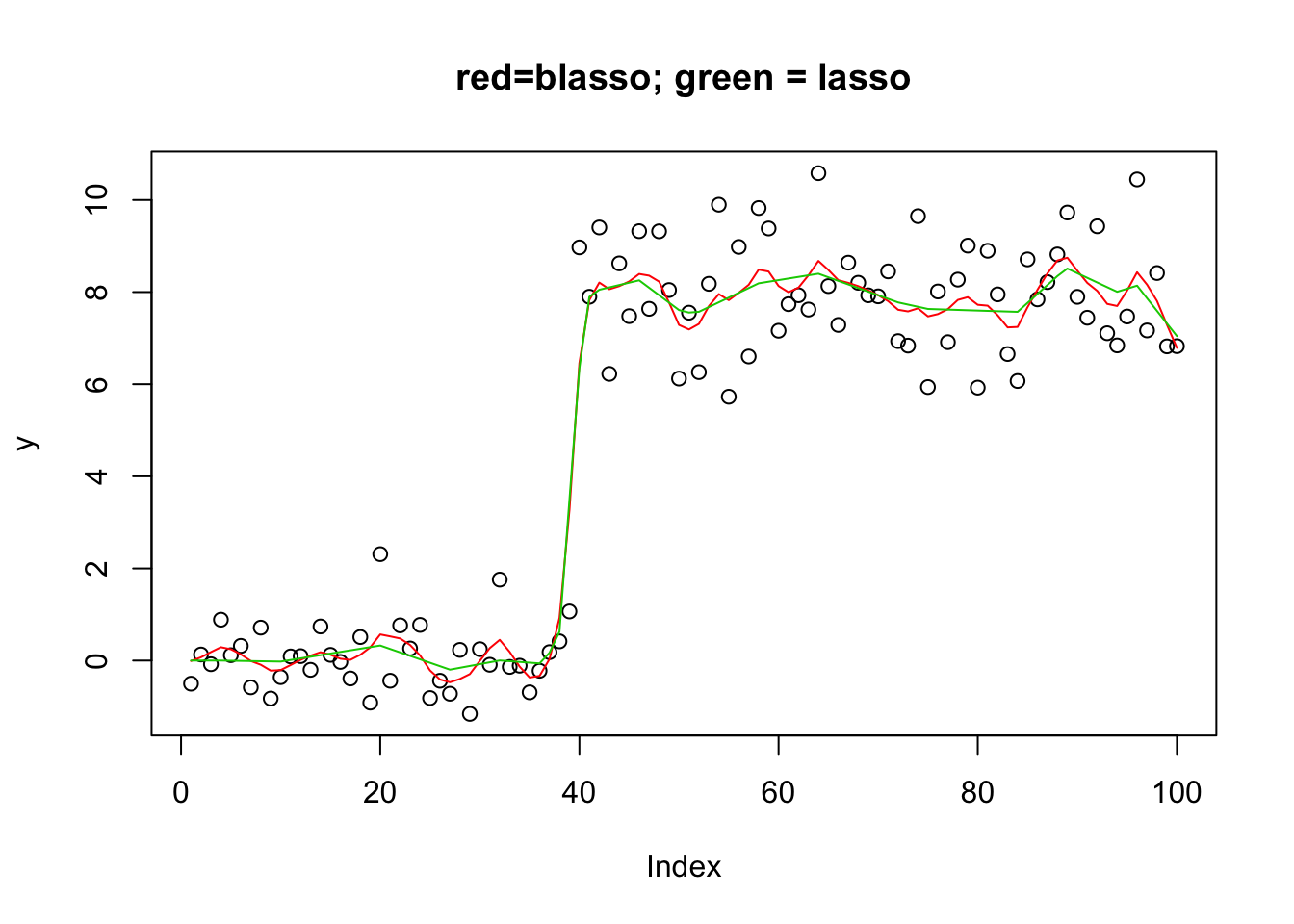
| Version | Author | Date |
|---|---|---|
| 99039f1 | Matthew Stephens | 2020-06-02 |
plot(y.em3$bhat,y.em2$bhat, xlab="blasso",ylab="lasso")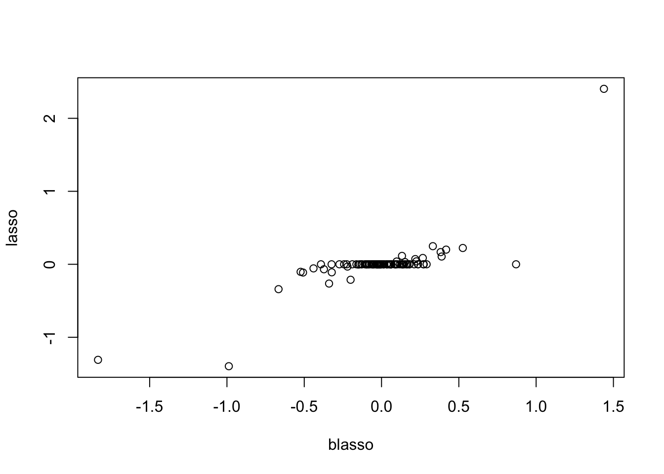
| Version | Author | Date |
|---|---|---|
| 99039f1 | Matthew Stephens | 2020-06-02 |
Check the posterior mode is same as my Lasso implementation
y.em4 = blasso_em(y,X,b.init = rnorm(100),1,1,100,compute_mode=TRUE)
plot(y)
lines(X %*% y.em4$bhat,col=2)
lines(X %*% y.em2$bhat,col=3)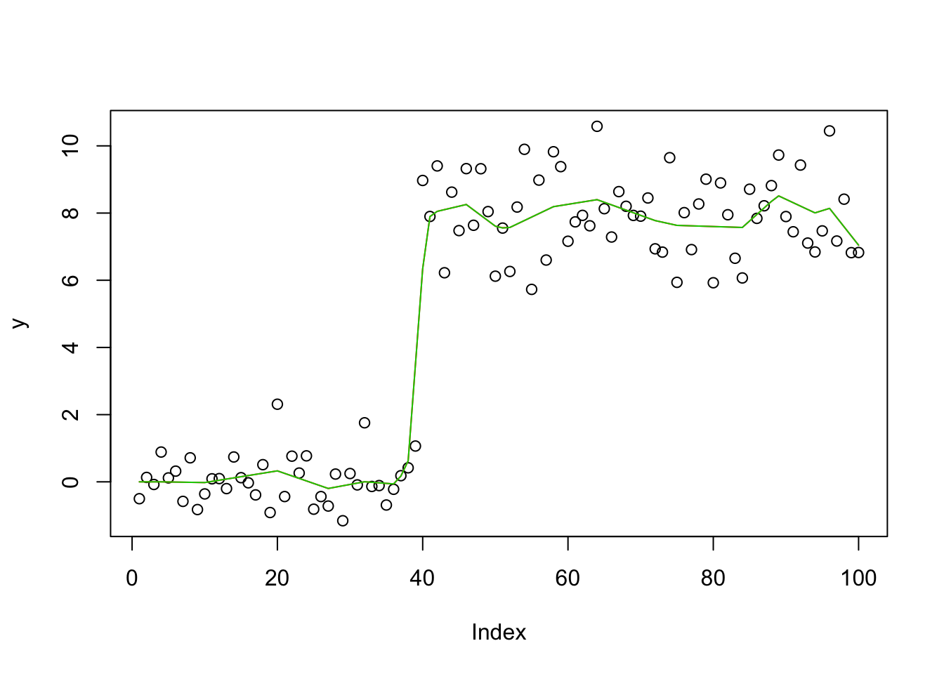
| Version | Author | Date |
|---|---|---|
| 99039f1 | Matthew Stephens | 2020-06-02 |
plot(y.em4$bhat,y.em2$bhat)
| Version | Author | Date |
|---|---|---|
| 99039f1 | Matthew Stephens | 2020-06-02 |
VEB lasso: estimate hyperparameters eta
The next step is to estimate/update the prior hyperparameter \(\eta\), and the residual variance \(s^2\). This becomes a “Variational Empirical Bayes” (VEB) approach.
The update for eta is rather simple: eta = mean(sqrt(diag(EB2))*sqrt(eta/2) + eta/2). Again see here.
The update for \(s^2\) is \[(1/n)E||y-Xb||^2_2\]. This could be simplified if we make a mean-field approximation on \(b\), but for now we just go with the full.
Note we are using the unscaled parameterization right now for simplicity. This may cause problems with multi-modality, as discussed here.
calc_s2hat = function(y,X,XtX,EB,EB2){
  n = length(y)
  Xb = X %*% EB
  s2hat = as.numeric((1/n)* (t(y) %*% y - 2*sum(y*Xb) + sum(XtX * EB2)))
}

# see objective computation for scaling of eta and residual variance s2
# if compute_mode=TRUE we have the regular LASSO
blasso_veb = function(y,X,b.init,s2=1,eta=1,niter=100){
  n = nrow(X)
  p = ncol(X)
  b = b.init # initiolize
  XtX = t(X) %*% X
  Xty = t(X) %*% y
  obj = rep(0,niter)
  EB = rep(1,p)
  EB2 = diag(p)

  for(i in 1:niter){
    W = as.vector(1/sqrt(diag(EB2) + EB^2) * sqrt(2/eta))

    V = chol2inv(chol(XtX+ diag(s2*W)))
    Sigma1 = s2*V  # posterior variance of b
    varB = diag(Sigma1)

    mu1 = as.vector(V %*% Xty) # posterior mean of b
    EB = mu1
    EB2 = Sigma1 + outer(mu1,mu1)

    eta = mean(sqrt(diag(EB2))*sqrt(eta/2) + eta/2)
    s2 = calc_s2hat(y,X,XtX,EB,EB2)
  }
  return(list(bhat=EB,eta=eta,s2 = s2))
}
Try it out on trend-filtering example:
set.seed(100)
sd = 1
n = 100
p = n
X = matrix(0,nrow=n,ncol=n)
for(i in 1:n){
  X[i:n,i] = 1:(n-i+1)
}
#X = X %*% diag(1/sqrt(colSums(X^2)))

btrue = rep(0,n)
btrue[40] = 8
btrue[41] = -8
y = X %*% btrue + sd*rnorm(n)

plot(y)
lines(X %*% btrue)

y.veb = blasso_veb(y,X,b.init = rnorm(100),1,1,100)
lines(X %*% y.veb$bhat,col=2)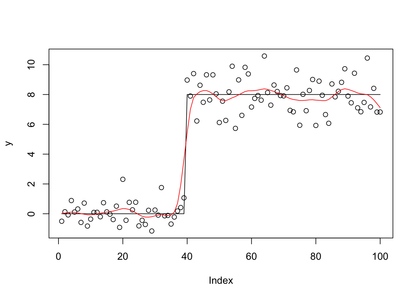
| Version | Author | Date |
|---|---|---|
| 328203f | Matthew Stephens | 2020-06-17 |
A dense simulation
Now a dense simulation, similar to here but with \(n\) and \(p\) ten times smaller to make it run fast. The idea here is that we know this case can cause convergence issues for VEB approach and we want to see if this affects the VEB lasso.
library(glmnet)Loading required package: MatrixLoaded glmnet 3.0-2 set.seed(123)
n <- 50
p <- 100
p_causal <- 50 # number of causal variables (simulated effects N(0,1))
pve <- 0.95
nrep = 10
rmse_blasso_veb = rep(0,nrep)
rmse_glmnet = rep(0,nrep)
for(i in 1:nrep){
sim=list()
sim$X = matrix(rnorm(n*p),nrow=n)
B <- rep(0,p)
causal_variables <- sample(x=(1:p), size=p_causal)
B[causal_variables] <- rnorm(n=p_causal, mean=0, sd=1)
sim$B = B
sim$Y = sim$X %*% sim$B
E = rnorm(n,sd = sqrt((1-pve)/(pve))*sd(sim$Y))
sim$Y = sim$Y + E
fit_blasso_veb <- blasso_veb(sim$Y,sim$X,b.init=rep(0,p))
fit_glmnet <- cv.glmnet(x=sim$X, y=sim$Y, family="gaussian", alpha=1, standardize=FALSE)
rmse_blasso_veb[i] = sqrt(mean((sim$B-fit_blasso_veb$bhat)^2))
rmse_glmnet[i] = sqrt(mean((sim$B-coef(fit_glmnet)[-1])^2))
}
plot(rmse_blasso_veb,rmse_glmnet, xlim=c(0.4,0.75),ylim=c(0.4,0.75), main="RMSE for glmnet vs blasso_veb, dense case")
abline(a=0,b=1)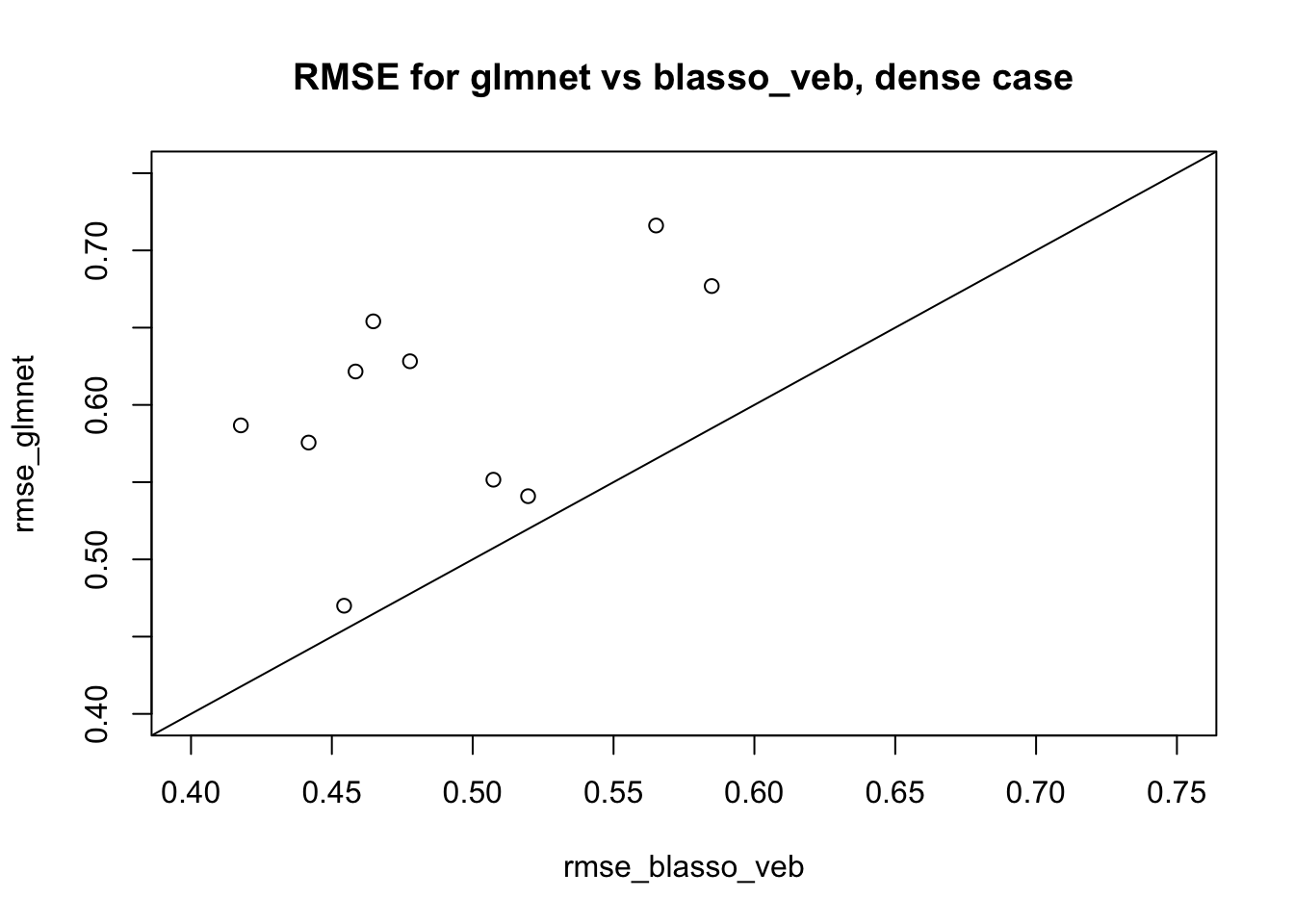
| Version | Author | Date |
|---|---|---|
| 6a34255 | Matthew Stephens | 2020-06-18 |
We see the results for blasso_veb are consistently better than glmnet here – reassuring, if ultimately kind of expected since the truth is quite dense. Interestingly there is no sign of convergence problems we could have seen.
Here I repeat with sparser. We see here that glmnet is sligthly better (also kind of expected).
  set.seed(123)
  n <- 50
  p <- 100
  p_causal <- 5 # number of causal variables (simulated effects N(0,1))
  pve <- 0.95
  nrep = 10
  rmse_blasso_veb = rep(0,nrep)
  rmse_glmnet = rep(0,nrep)

  for(i in 1:nrep){
    sim=list()
    sim$X =  matrix(rnorm(n*p),nrow=n)

    B <- rep(0,p)
    causal_variables <- sample(x=(1:p), size=p_causal)
    B[causal_variables] <- rnorm(n=p_causal, mean=0, sd=1)

    sim$B = B
    sim$Y = sim$X %*% sim$B
    E = rnorm(n,sd = sqrt((1-pve)/(pve))*sd(sim$Y))
    sim$Y = sim$Y + E

    fit_blasso_veb <- blasso_veb(sim$Y,sim$X,b.init=rep(0,p))

    fit_glmnet <- cv.glmnet(x=sim$X, y=sim$Y, family="gaussian", alpha=1, standardize=FALSE)


    rmse_blasso_veb[i] = sqrt(mean((sim$B-fit_blasso_veb$bhat)^2))
    rmse_glmnet[i] = sqrt(mean((sim$B-coef(fit_glmnet)[-1])^2))

  }

  plot(rmse_blasso_veb,rmse_glmnet,  main="RMSE for glmnet vs blasso_veb, sparse case", xlim=c(0,.1),ylim=c(0,.1))
  abline(a=0,b=1)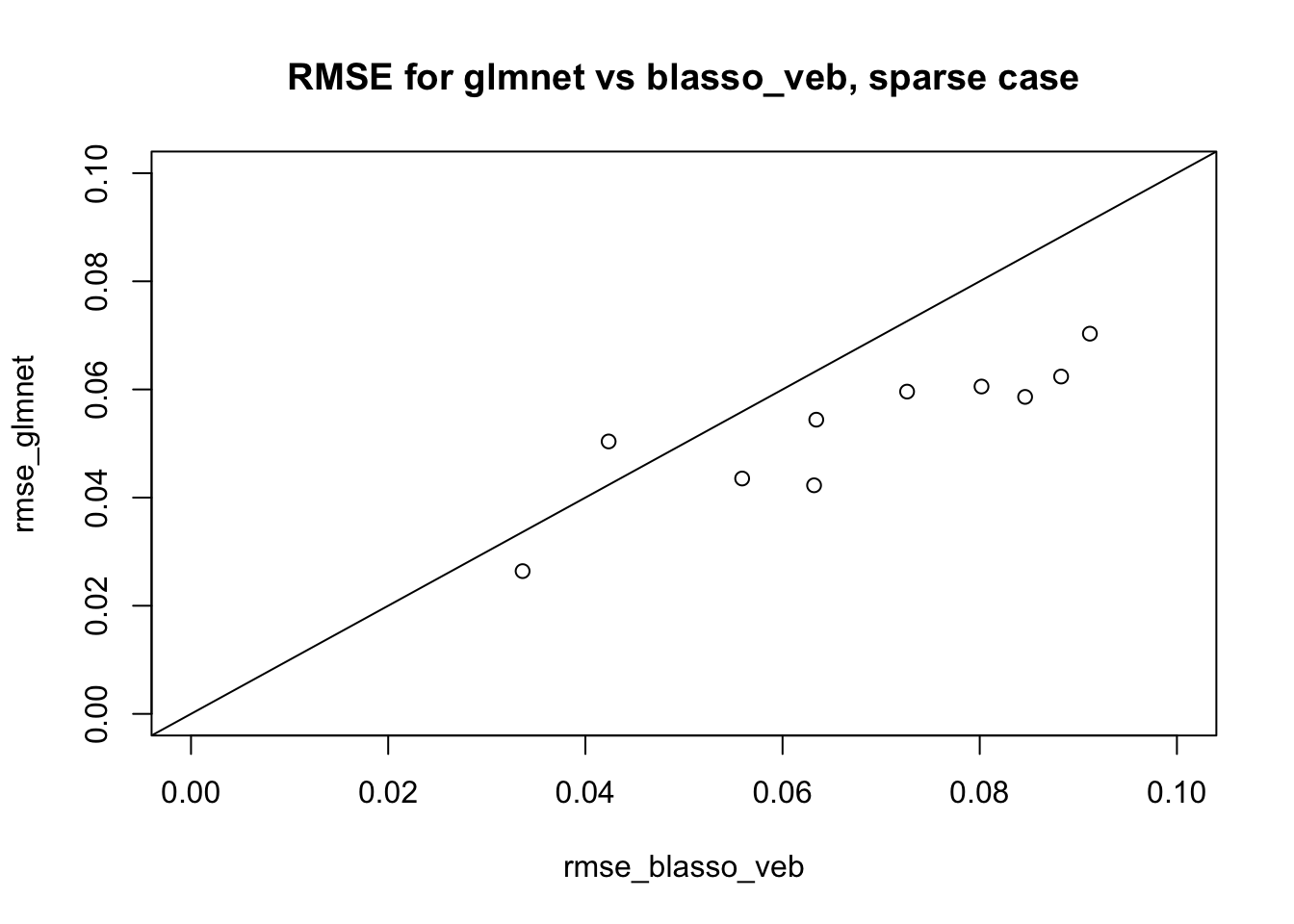
| Version | Author | Date |
|---|---|---|
| 6a34255 | Matthew Stephens | 2020-06-18 |
sessionInfo()R version 3.6.0 (2019-04-26)
Platform: x86_64-apple-darwin15.6.0 (64-bit)
Running under: macOS Mojave 10.14.6
Matrix products: default
BLAS: /Library/Frameworks/R.framework/Versions/3.6/Resources/lib/libRblas.0.dylib
LAPACK: /Library/Frameworks/R.framework/Versions/3.6/Resources/lib/libRlapack.dylib
locale:
[1] en_US.UTF-8/en_US.UTF-8/en_US.UTF-8/C/en_US.UTF-8/en_US.UTF-8
attached base packages:
[1] stats graphics grDevices utils datasets methods base
other attached packages:
[1] glmnet_3.0-2 Matrix_1.2-18
loaded via a namespace (and not attached):
[1] Rcpp_1.0.4.6 knitr_1.28 whisker_0.4 magrittr_1.5
[5] workflowr_1.6.1 lattice_0.20-40 R6_2.4.1 rlang_0.4.5
[9] foreach_1.4.8 stringr_1.4.0 tools_3.6.0 grid_3.6.0
[13] xfun_0.12 git2r_0.26.1 iterators_1.0.12 htmltools_0.4.0
[17] yaml_2.2.1 digest_0.6.25 rprojroot_1.3-2 later_1.0.0
[21] codetools_0.2-16 promises_1.1.0 fs_1.3.2 shape_1.4.4
[25] glue_1.4.0 evaluate_0.14 rmarkdown_2.1 stringi_1.4.6
[29] compiler_3.6.0 backports_1.1.5 httpuv_1.5.2